9.1 Multinomial Distribution

Recall that the binomial distribution arises from a random experiment where the outcome is binary black and white, postive or negative, or yes and no. Hence, a natural generalization of the binomial arises when we model the outcome of a random experiment with \(k(>2)\) possible outcomes, with each having probability \(p_i\), \(i=1,\ldots,k\). We denote these probabiities as a \(k\)-dimensional non-negative vector \(\tilde{p}\), we note that \(\tilde{p}^{\scriptscriptstyle\mathsf{T}}\tilde{1}=1\) (superscript \(\mathsf{T}\) denotes transpose). Let \((X_{1,1},\ldots,X_{1,k})\) denote the vector which indicates the outcome of a single such experiment; for example, if the outcome was of the \(j\)-th type, then \(X_{1,j}=1\) and the rest of the coordinates zero. This is the simplest random vector one can think of, so let us analyze some of its properties.

First we note that by classifying the outcome as either of type \(j\) or not, we return to the setting of binary outcomes. In other words, \(X_{1,j}\) is a Bernoulli random variable with \({\rm Pr}\left(X_{1,j}=1\right)=p_j\). Hence we get

\[ \mathbb{E}{\left(X_{1,j}\right)}=1, \quad \hbox{and} \quad {\rm Var}\left(X_{1,j}\right)=p_j(1-p_j). \] Also, note that since the outcome is of exactly one type, \(X_{1,i}X_{1,j}\equiv 1\). This implies that

\[ {\rm Cov}\left(X_{1,i},X_{1,j}\right)=\mathbb{E}{\left(X_{1,i}X_{1,j}\right)}- \mathbb{E}{\left(X_{1,i}\right)}\mathbb{E}{\left(X_{1,j}\right)}=0-p_ip_j=-p_ip_j. \]

To summarize, we get that the variance-covariance matrix \(\Sigma\) is given by

\[ \begin{aligned} \Sigma&:= \begin{pmatrix} p_1(1-p_1) & -p_1p_2 & \cdots & -p_1p_k \\ -p_2p_1 & p_2(1-p_2) & \cdots & -p_2p_k \\ \vdots & \vdots & \ddots & \vdots\\ -p_kp_1 & -p_kp_2 & \cdots & p_k(1-p_k) \\ \end{pmatrix} \end{aligned} \]

The multinomial distribution is the distribution of the vector that represents the counts of the number of outcomes of each type from \(n\) independent repetitions of the above random experiment. In other words, it is the distribution of the vector \[ \tilde{X}:=\left(\sum_{i=1}^n X_{i,1},\ldots,\sum_{i=1}^n X_{i,k}\right). \] From the above we conclude that

\[ \mathbb{E}{\left(\tilde{X}\right)}=n\tilde{p}, \quad \hbox{and} \quad \mathbb{E}{\left((\tilde{X}-\tilde{p})(\tilde{X}-\tilde{p})^{\scriptscriptstyle\mathsf{T}}\right)}=n\Sigma. \] Also, it probability mass function is given by

\[ {\rm Pr}\left(\tilde{X}=\tilde{x}\right)=\frac{n!}{\prod_{j=1}^k x_j!} \prod_{j=1}^k p_j^{x_j}, \quad \tilde{x}\geq 0, \tilde{x}^{\scriptscriptstyle\mathsf{T}}\tilde{1}=n. \] and these can be simulated directly by using rmultinom and indirectly by using sample (How?).

9.2 Some Linear Algebraic Observations

Some linear algebraic observations that will be useful below. We start by observing that,

\[ \begin{aligned} \Sigma&=\mathbf{diag}(\tilde{p}) - \tilde{p}\tilde{p}^{\scriptscriptstyle\mathsf{T}}\\ &= \mathbf{diag}\left(\sqrt{\tilde{p}}\right)\left(I-\sqrt{\tilde{p}}\sqrt{\tilde{p}}^{\scriptscriptstyle\mathsf{T}}\right)\mathbf{diag}\left(\sqrt{\tilde{p}}\right). \end{aligned} \] In the above, let us denote by \(P\) the matrix \(\left(I-\sqrt{\tilde{p}}\sqrt{\tilde{p}}^{\scriptscriptstyle\mathsf{T}}\right)\). Note that \(P\) is a symmetric matrix that satisfies,

\[ \begin{aligned} P^2&=\left(I-\sqrt{\tilde{p}}\sqrt{\tilde{p}}^{\scriptscriptstyle\mathsf{T}}\right)\left(I-\sqrt{\tilde{p}}\sqrt{\tilde{p}}^{\scriptscriptstyle\mathsf{T}}\right)\\ &=I-2\sqrt{\tilde{p}}\sqrt{\tilde{p}}^{\scriptscriptstyle\mathsf{T}}+\sqrt{\tilde{p}}\sqrt{\tilde{p}}^{\scriptscriptstyle\mathsf{T}}\sqrt{\tilde{p}}\sqrt{\tilde{p}}^{\scriptscriptstyle\mathsf{T}}\\ &=I-\sqrt{\tilde{p}}\sqrt{\tilde{p}}^{\scriptscriptstyle\mathsf{T}}=P, \end{aligned} \]

since \(\sqrt{\tilde{p}}^{\scriptscriptstyle\mathsf{T}}\sqrt{\tilde{p}}=1\).

Matrices that satisfy \(A^2=A\) are called idempotent. Note that this implies that the columns of \(A\) are eigen vectors of \(A\), and their corresponding eigen values are equal to one. Moreover, since \(A^{\scriptscriptstyle\mathsf{T}}=A\). Hence, we see that vectors orthogonal to the column space are annulled by \(A\), i.e these form eigen vectors corresponding to zero eigen values. In other words, we have shown that symmetric idempotent matrix represent orthogonal projections onto its column space. Note that we know that \({\mathrm{Tr}\left(A\right)}\) equals the sum of the eigen values; in the case of the symmetric idempotent matrix, since the eigen values are zero/one, \({\mathrm{Tr}\left(A\right)}\) equals the rank of \(A\), which in turn equals the dimension of its column space. Putting it together, we see that symmetric idempotent matrices represent linear transformations that project vectors to its column space of rank equal to its trace.

What does the above imply about \(P\). Note that \(P\) above is a symmetric idempotent matrix, and

\[ {\mathrm{Tr}\left(I-\sqrt{\tilde{p}}\sqrt{\tilde{p}}^{\scriptscriptstyle\mathsf{T}}\right)}={\mathrm{Tr}\left(I\right)}-{\mathrm{Tr}\left(\sqrt{\tilde{p}}\sqrt{\tilde{p}}^{\scriptscriptstyle\mathsf{T}}\right)}=k-{\mathrm{Tr}\left(\sqrt{\tilde{p}}^{\scriptscriptstyle\mathsf{T}}\sqrt{\tilde{p}}\right)}=k-1. \]

In the above we used the fact that \({\mathrm{Tr}\left(AB\right)}={\mathrm{Tr}\left(BA\right)}\). In fact, \(P\) projects onto the orthogonal space of the unidimensional subspace containing \(\sqrt{\tilde{p}}\).

Now by the eigendecomposition of a symmetric matrix we know that \(P\) can be written as \(Q\Lambda Q^{\scriptscriptstyle\mathsf{T}}\), where \(Q\) is an orthogonal matrix, and \(\Lambda\) is a diagonal matrix with the eigen values of \(P\) as its diagonal. Using the fact that \(P\) has \(k-1\) eigen values equal to \(1\) and one zero eigen value, we can assume that, by permuting if necessary, that \(\Lambda=\mathbf{diag}((1,\ldots,1,0))\).

9.3 Asymptotic Theory

Note from the above development that \(\tilde{X}\), a vector with a multinomial distribution with parameter \(n\) and \(\tilde{p}\), is a sum of iid vectors with the common distribution being the multinomial with parameter \(1\) and \(\tilde{p}\). Hence, we can invoke the multivariate Central Limit Theorem to conclude that

\[ \frac{1}{\sqrt{n}}\left(\tilde{X}-\mathbb{E}{\left(\tilde{X}\right)}\right)\buildrel {\rm d} \over \longrightarrow N_k(\tilde{0},\Sigma), \] where \(\Sigma\) is as defined above. Note that the convergence happens as \(n\) approaches infinity. Now from the above we have that,

\[ (\mathbf{diag}(\sqrt{\tilde{p}}))^{-1}\Sigma (\mathbf{diag}(\sqrt{\tilde{p}})^{\scriptscriptstyle\mathsf{T}})^{-1}=P. \] Hence defining \(\tilde{Z}\) by

\[ \tilde{Z}:=\frac{1}{\sqrt{n}}(\mathbf{diag}(\sqrt{\tilde{p}}))^{-1}\left(\tilde{X}-\mathbb{E}{\left(\tilde{X}\right)}\right), \] we have

\[ \tilde{Z}\buildrel {\rm d} \over \longrightarrow N_k(\tilde{0},P). \] Now, further by using the fact that \(P=Q\Lambda Q^{\scriptscriptstyle\mathsf{T}}\), we have that

\[ Q^{\scriptscriptstyle\mathsf{T}}\tilde{Z}\buildrel {\rm d} \over \longrightarrow N_k(\tilde{0},\Lambda)\buildrel \rm d \over =(N_{k-1}(\tilde{0},I_{(k-1)\times(k-1)}),0). \] The above, in particular, and the fact that \(Q\) is an orthogonal matrix implies that

\[ \begin{aligned} \tilde{Z}^{\scriptscriptstyle\mathsf{T}}\tilde{Z}&={\mathrm{Tr}\left(\tilde{Z}\tilde{Z}^{\scriptscriptstyle\mathsf{T}}\right)}\\ &={\mathrm{Tr}\left(\tilde{Z}Q^{\scriptscriptstyle\mathsf{T}}Q\tilde{Z}^{\scriptscriptstyle\mathsf{T}}\right)}\\ &=Q^{\scriptscriptstyle\mathsf{T}}\tilde{Z}^{\scriptscriptstyle\mathsf{T}}Q^{\scriptscriptstyle\mathsf{T}}\tilde{Z}\\ &\buildrel \rm d \over =\tilde{Y}^{\scriptscriptstyle\mathsf{T}}\tilde{Y}\\ &\buildrel \rm d \over =\chi^2_{k-1}, \end{aligned} \] where \(Y\sim N_{k-1}(\tilde{0},I_{(k-1)\times(k-1)})\). Below we confirm this by simulation for \(k=3\) and \(n=50\).

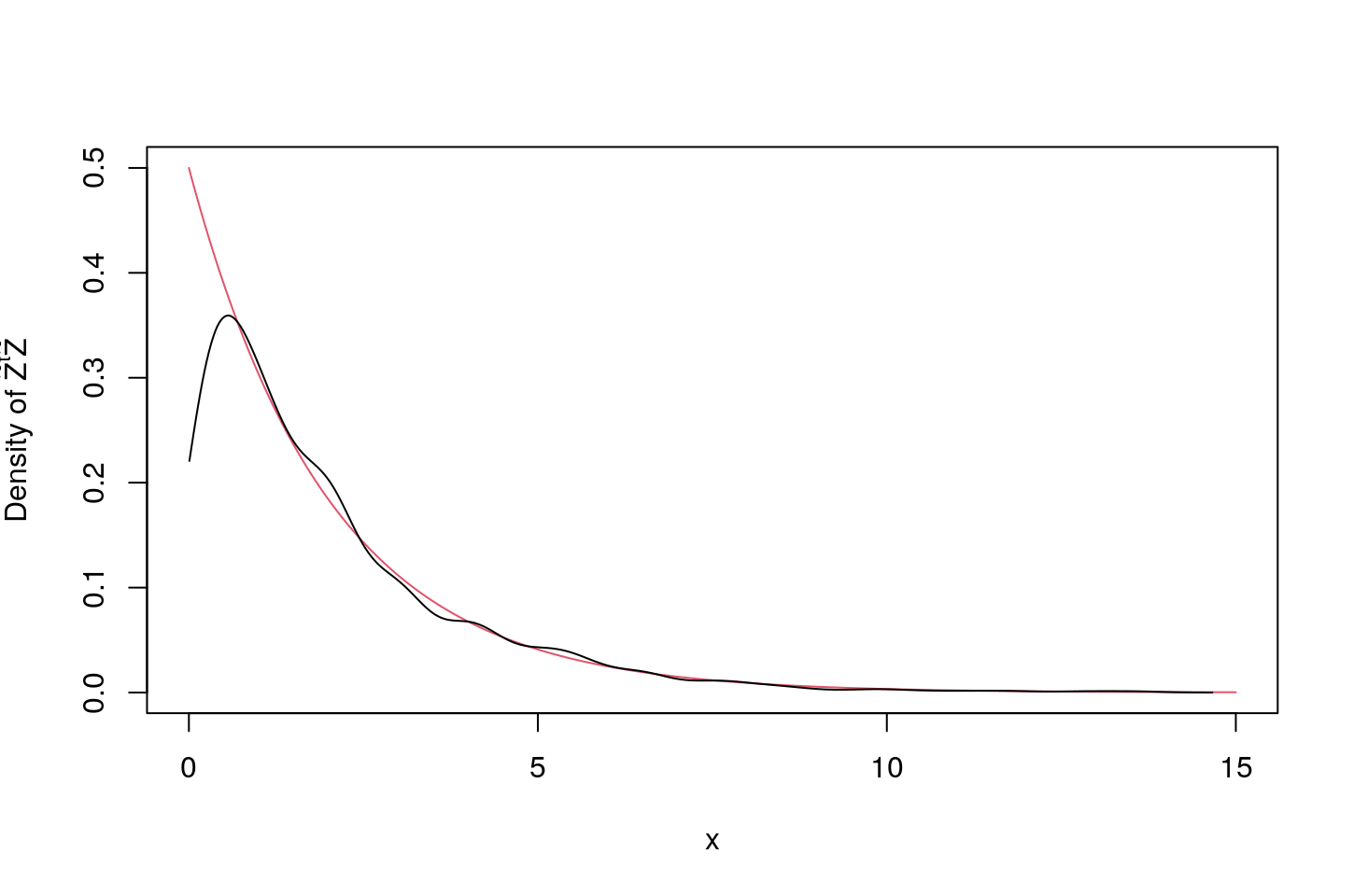
9.4 Chi-squared Test

Consider a grouped data set of size \(n\) with \(k\) groups, and sample proportions \(\hat{p}_j\), \(j=1,\ldots, k\). Let the sample proportion vector be denoted by \(\hat{p}\). We use the notation of the text, and denote the \(j\)-th group be defined by the interval \((c_{j-1},c_j]\), with \(0=c_0<c_1 \ldots<c_k=\infty\). Now suppose that we wish to test if the true distribution is \(F\). Now by defining \(p_j:=F(c_j)-F(c_{j-1})\), \(j=1,\ldots, k\), we immediately see that

\[ \hat{p}\buildrel \rm d \over =\frac{1}{n}\tilde{X}. \]

Hence, we get that

\[ \begin{aligned} \chi^2&=\sum_{j=1}^k \frac{n(\hat{p}_j-p_j)^2}{p_j}\\ &=\sum_{j=1}^k \left(\frac{\sqrt{n}(\hat{p}_j-p_j)}{\sqrt{p_j}}\right)^2\\ &\buildrel \rm d \over =\tilde{Z}^{\scriptscriptstyle\mathsf{T}}\tilde{Z}\\ &\buildrel \rm d \over =\chi^2_{k-1}. \end{aligned} \]