5 MLE Computation
In mathematical statistics we predominantly, if not completely, restrict ourselves to consider models where the estimators permit closed form expressions. This serves a purpose as it allows for the focus to be on the statistical principles involved, and prevents diverting attention to the computational aspects of calculating the MLE that arise in more realistic models. Also, such courses do not consider data that are truncated or censored; such data are in fact the more common ones in medicine/biostatistics and also in actuarial science. In this note I will expose you to some tools in R that may be useful in computing the MLE in such situations.
5.1 Gamma with unknown shape
This example deals with the Data Set B of the text which is supposed to represent twenty workers compensation medical benefit claims. The data is presented in the tables below - I demonstrate the use of two packages to nicely tabulate your data.
library("kableExtra")
med_claims <- c(27, 82, 115, 126, 155, 161, 243, 294, 340, 384, 457, 680, 855, 877, 974, 1193, 1340, 1884, 2558, 15743);
med_claims_df<-data.frame("Medical Claims"=med_claims <- c(27, 82, 115, 126, 155, 161, 243, 294, 340, 384, 457, 680, 855, 877, 974, 1193, 1340, 1884, 2558, 15743));
med_claims_df%>%
  kable() %>%
  kable_styling() %>%
scroll_box(width = "100px", height = "200px")| Medical.Claims |
|---|
| 27 |
| 82 |
| 115 |
| 126 |
| 155 |
| 161 |
| 243 |
| 294 |
| 340 |
| 384 |
| 457 |
| 680 |
| 855 |
| 877 |
| 974 |
| 1193 |
| 1340 |
| 1884 |
| 2558 |
| 15743 |
library(xtable);
tab<-xtable(t(med_claims_df),caption="Data Set B: Workers Compensation Medical Claims",table.placement="H",type="html",digits=c(0));
print(tab, type="html")| 1 | 2 | 3 | 4 | 5 | 6 | 7 | 8 | 9 | 10 | 11 | 12 | 13 | 14 | 15 | 16 | 17 | 18 | 19 | 20 | |
|---|---|---|---|---|---|---|---|---|---|---|---|---|---|---|---|---|---|---|---|---|
| Medical.Claims | 27 | 82 | 115 | 126 | 155 | 161 | 243 | 294 | 340 | 384 | 457 | 680 | 855 | 877 | 974 | 1193 | 1340 | 1884 | 2558 | 15743 |
The gamma family of distributions is chosen as a model for this data, and the goal is to estimate the unknown shape and scale parameters. Just to fix the parametrization, the density is given by \[ f_{\alpha,\theta}(x)=\frac{1}{\Gamma(\alpha)\theta^\alpha} e^{-(x/\theta)} x^{\alpha-1 },\quad x\geq 0; \] the parameter space is given by \((0,\infty)^2\). We note that, the log-likelihood is given by, \[ l(\alpha,\theta):=-n\log\Gamma(\alpha) - n\alpha\log\theta - \frac{1}{\theta}\sum_{i=1}^n x_i +(\alpha-1)\sum_{i=1}^n \log x_i. \] Note that \[ \frac{\partial }{\partial \theta}l(\alpha,\theta) =-\frac{n\alpha}{\theta} +\frac{1}{\theta^2}\sum_{i=1}^n x_i, \] and equating it to zero yields, \[ \hat{\theta}_{MLE}= \frac{\bar{x}}{\hat{\alpha}_{MLE}}. \] This is so as \[ \frac{\partial^2 }{\partial \theta^2}l(\alpha,\theta)\Bigg\vert_{(\alpha=\hat{\alpha}_{MLE},\theta=\hat{\theta}_{MLE})} =\frac{n\hat{\alpha}_{MLE}}{\hat{\theta}_{MLE}^2} -\frac{2}{\hat{\theta}_{MLE}^3}\sum_{i=1}^n x_i=\frac{n\hat{\alpha}_{MLE}}{\hat{\theta}_{MLE}^3} \left(\hat{\theta}_{MLE}-\frac{2\bar{x}}{\hat{\alpha}_{MLE}}\right) = -\frac{n\hat{\alpha}_{MLE}}{\hat{\theta}_{MLE}^2} <0. \]
While we have an expression for \(\hat{\theta}_{MLE}\), it involves an unknown - \(\hat{\alpha}_{MLE}\). The nice thing about it is that it still helps reduce the optimization problem from one on \(\mathbb{R}_+^2\) to \(\mathbb{R}_+\). This is so because we reduce the optimization problem to that of maximizing \[ \begin{aligned} l(\alpha,\bar{x}/\alpha)&:=-n\log\Gamma(\alpha) - n\alpha\log\frac{\bar{x}}{\alpha} - \frac{\alpha}{\bar{x}}\sum_{i=1}^n x_i +(\alpha-1)\sum_{i=1}^n \log x_i\\ &=-n\log\Gamma(\alpha) - n\alpha\log{\bar{x}}+ n\alpha\log{\alpha} - n\alpha + (\alpha-1)\sum_{i=1}^n \log x_i. \end{aligned} \]
optimize function as follows:
# Sufficient Statistics
  xbar<-mean(med_claims);
  sum_logx<-sum(log(med_claims));
  n<-length(med_claims);
# Loglikelihood
  like<-function(a){
    -n*lgamma(a)-n*a*(log(xbar/a)+1)+(a-1)*sum_logx
  }
opt<-optimize(like,c(0.1,4),maximum=TRUE);
# MLE for alpha, theta and the value of the loglikelihood - See Example 13.4 in the text
round(c(opt$maximum,xbar/opt$maximum,opt$objective),6)
## [1] 0.556165 2561.111354 -162.293403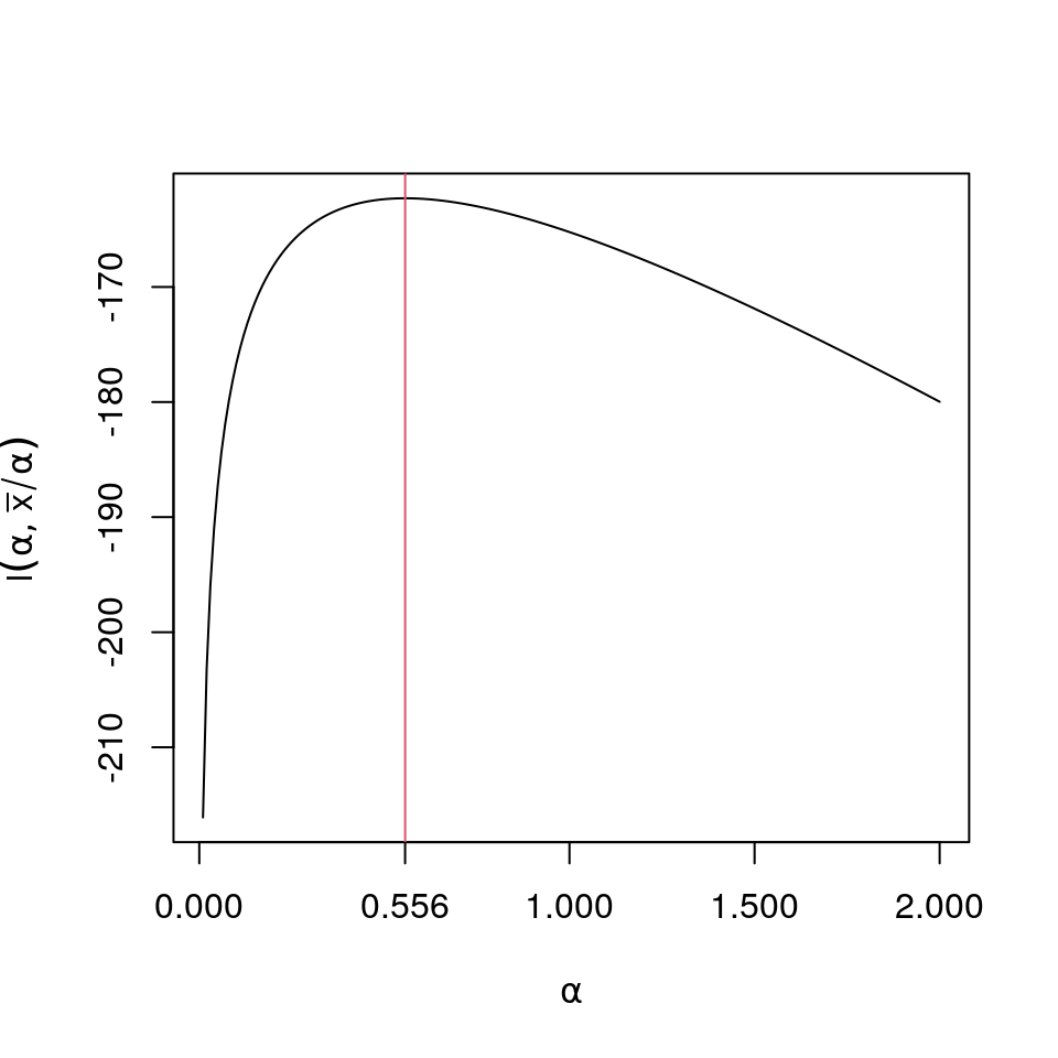
plot(a<-(1:200)/100,sapply(a,like),type="l",ylab=expression(l(alpha,bar(x)/alpha)),xlab=expression(paste(alpha)),xaxt="n");
axis(1,at=round(c(0,opt$maximum,1,1.5,2),3))
lines(rep(opt$maximum,201),-160-40*(0:200)/100,col=2)
An alternate method is to find the root of \[ \begin{aligned} \frac{\partial}{\partial\alpha}l(\alpha,\bar{x}/\alpha)&= -n\frac{\Gamma'(\alpha)}{\Gamma(\alpha)} - n\log{\bar{x}}+ n\log{\alpha} + \sum_{i=1}^n \log x_i\\ &=n\left(-\frac{\Gamma'(\alpha)}{\Gamma(\alpha)} - \log{\bar{x}}+ \log{\alpha} + \frac{1}{n}\sum_{i=1}^n \log x_i\right) \end{aligned} \] Some comments on the expression within the brackets:
Note that the expression is scale invariant i.e. we can wolog assume that \(\theta=1\) (Why?). Now observe that for a \(Gamma(\alpha,1)\) random variable \(X\),
\[ \mathbb{E}\left({log(X)}\right)=\frac{\Gamma'(\alpha)}{\Gamma(\alpha)},\quad \hbox{and} \quad \mathbb{E}\left({X}\right)=\alpha. \]
The above comment implies that we seek a root of (with both sides being non-negative by Jensen’s inequality)
\[ \log{\mathbb{E}_\alpha\left({X}\right)} -\mathbb{E}_\alpha\left({log(X)}\right) = \left(\log{\bar{x}} - \frac{1}{n}\sum_{i=1}^n \log x_i \right) \]
Finally we note that by Jensen’s inequality (as \(log\) is a concave function) both sides of the above equation are non-negative. We below use these comments to implement another algorithm to find \(\hat{\alpha}_{MLE}\) - this uses the digamma function.
# The rhs
  rhs<-log(xbar)-sum_logx/n;
# The lhs - using the digamma function
  like_der<-function(a){
    log(a)-digamma(a)-rhs
  }
amle<-uniroot(like_der,interval=c(0.01,4))$root
# MLE for alpha, theta
round(c(amle,xbar/amle),6)
## [1] 0.556173 2561.075759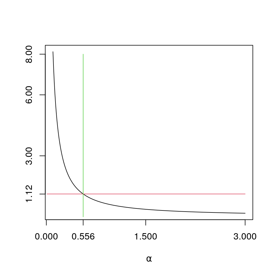
plot(a<-(10:300)/100,sapply(a,like_der)+rhs,type="l",xlab=expression(paste(alpha)),ylab="",yaxt="n",xaxt="n")
#plot(a<-(1:200)/100,sapply(a,like),type="l",xlab=expression(paste(alpha)),xaxt="n");
axis(2,at=round(c(rhs,3,6,8),2))
lines((1:300)/100,rep(rhs,300),col=2)
lines(rep(amle,9),0:8,col=3)
axis(1,at=round(c(0,opt$maximum,1.5,3),3))
5.2 Grouped Data
In this example we will look at the analysis of Data Set C in the text which represents 227 payments from a general liability insurance policy block. The data set is given below (see Example 13.5 of the text).
library("kableExtra")
genliab_df<-data.frame("Lower End Point"=c(0,7500,17500,32500,67500,125000,300000),"Upper End Point"=c(7500,17500,32500,67500,125000,300000,Inf), "Payments"=c(99,42,29,28,17,9,3));
genliab_df%>%
  kable(caption="General Liability Payments - Data Set C") %>%
kable_styling(bootstrap_options = c("striped", "hover"),full_width=F,position="float_right") | Lower.End.Point | Upper.End.Point | Payments |
|---|---|---|
| 0 | 7500 | 99 |
| 7500 | 17500 | 42 |
| 17500 | 32500 | 29 |
| 32500 | 67500 | 28 |
| 67500 | 125000 | 17 |
| 125000 | 300000 | 9 |
| 300000 | Inf | 3 |
This data set is an example of a grouped data set. We fit an exponential model to this. First, we realize that since the exponential is a scale family, we can change the unit to \(\$10,000\), estimate the scale parameter \(\theta\) and scale it back by a \(10,000\). To find the MLE we need the likelihood - we write a function and plot it below.
loglike<-function(theta){
  sum(genliab_df$Payments*log(exp(-genliab_df$Lower.End.Point/(theta*10000))-exp(-genliab_df$Upper.End.Point/(theta*10000))))
}
# Calculate some rough estimate for the range of optimization
sum((genliab_df$Lower.End.Point+genliab_df$Upper.End.Point)[-7]/20000*genliab_df$Payments[-7])/224;
## [1] 2.933036c("MLE of theta",round(mletheta<-optimize(loglike,c(0.5,5),maximum=TRUE)$maximum*10000,2))## [1] "MLE of theta" "29720.74"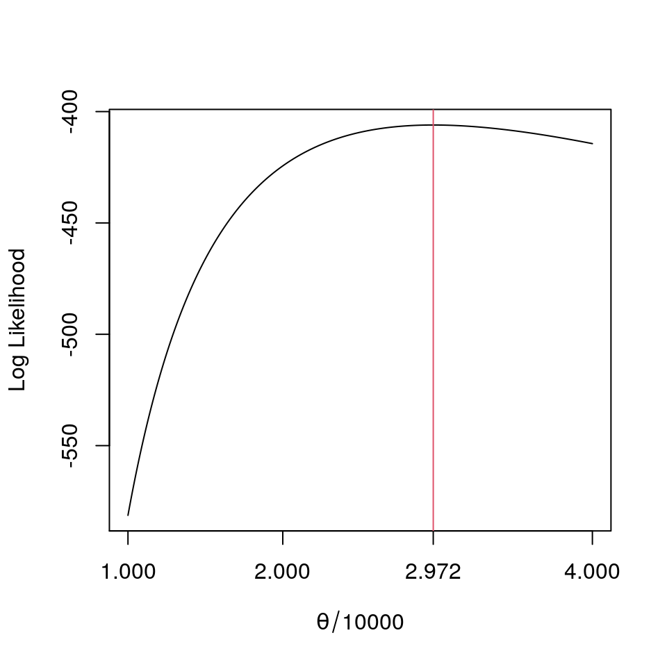
plot(a<-(100:400)/100,sapply(a,loglike),type="l",ylab="Log Likelihood",xlab=expression(paste(theta/10000)),xaxt="n");
axis(1,at=round(c(0,1,2,mletheta/10000,4),3))
lines(rep(mletheta/10000,11),-1000*(0:10),col=2)