3 Approximating a Compound Distribution
The goal of this note is to compare the normal and the log-normal approximations to a compound distribution. We will work in the setting where the common distribution of the \(X_i\)’s is a continuous distribution with support on \((0,\infty)\), and that \(\mathrm{Pr}\left(N=0\right)=0\); \(S:=\sum_{i=1}^N X_i\) is then a continuous random variable.
Specifically, we will take \(N\) to be a zero-truncated Poisson with parameter \(\lambda=3\) and \(X_i\)’s as i.i.d. (and independent of \(N\)) from a two-parameter Pareto distribution with \(\theta=1\) (think in terms of thousand dollars as the unit) and shape parameter \(\alpha=5\).
First, we will discuss simulating a compound random variable. But since our setup involves a truncated distribution we begin with a discussion of rejection sampling.
3.1 Recursive Rejection Sampling - Simulating from a Truncated Poisson
Let us suppose that you are simulating from some distribution \(F\) and that you are truncating to an interval \((l,u)\), with probability of a random variable \(X\sim F\) taking values in it equal to \(p_a\). Consider the problem of simulating \(n\) variables from this truncated distribution. Note that if we simulate \(m\) variables from \(F\), the number left after rejecting those outside \((l,u)\) is a \(Bin(m,p_a)\) random variable. Consider the problem of coming up with the value for \(m\) such that there is at least a probability of \(p_s\) that we would have accepted \(n\) of them. Using a normal approximation to the binomial, since \(n\) is usually high which implies \(m\) is high as well, we have \[m=\left\lceil \frac{n}{p_a} + a\sqrt{\left(\frac{a}{2p_a}\right)^2+\frac{n}{p_a}} +\frac{a^2}{2p_a}\right\rceil,\] where \(a=\Phi^{-1}(p_s)\sqrt{p_a(1-p_a)}\). It will be instructive to establish this - an elementary exercise in algebra and probability. Let us check it with zero-truncated Poisson with mean \(3\) - I use \(n=100\) but try it for higher values.
# The above formula wrapped in a function
mfunc<-function(n,pa,ps){
  a<-qnorm(ps)*sqrt(pa*(1-pa));
  ceiling(n/pa + a*sqrt((a/(2*pa))^2+n/pa) + a^2/(2*pa^2))
}

lambda<-3;
pa<-1-exp(-lambda);
n<-100;
ps<-0.75;
m<-mfunc(n,pa,ps);

# Check if it
f<-function(m){
  x<-rpois(m,lambda);
  sum(x>0)
}
x<-sapply(rep(m,100000),f);
c(mean(x>n), mean(x>=n)) # Encouraging if pa belongs to this interval
## [1] 0.71563 0.83551But this does not end the story. As there is a probability of \(1-ps\) that we may need more simulated values. So let us suppose we use the algorithm of repeating this for the remaining values we need until we have our \(n\) simulated values in total. This is a recursive implementation of the above algorithm.
truncsim<-function(n,pa,ps,FUN1=runif,l=0,u=1){
  m<-mfunc(n,pa,ps);
  x<-FUN1(m);
  x<-x[((x>l) & (x<u))]; # Note that we use the open interval (l,u)
  if (length(x)>=n) {
    x[1:n]
  }
  else {
    c(x,truncsim(max(n-length(x),1000),pa,ps,FUN1,l,u)) # I am using max(,1000) to minimize iterations with a low sample size
  }
}
# Check - Simulating Sero Truncated Poisson
x<-truncsim(10000,pa,ps,function(n){rpois(n,lambda)},0,Inf)
c(length(x),mean(x),lambda/pa) # We should see the first coordinate being n and the rest two ~equal by LLN
## [1] 10000.000000 3.116100 3.157187It is important to note that we have a free parameter - \(p_s\). Try to experiment with various choices, and post on Piazza your recommendation for \(p_s\).
3.2 Simulating a Compound Random Variable
Now that we have an efficient way of simulating zero-truncated Poissons, we need to simulated the required number of Pareto random variables to simulated the compound random variable. This is done below - we simulate a sample of \(10000\) compound random variables.
n<-10000; #Sample Size

# Simulating the zero truncated Poissons
lambda<-3; # Poisson Mean
pa<-1-exp(-lambda); # Probability of acceptance
ps<-0.75; # Probability of Simulating enough
N<-truncsim(10000,pa,ps,function(n){rpois(n,lambda)},0,Inf) # Checked above!!

# Simulating Paretos
theta<-1;
alpha<-5;
simPareto<-function(n,alpha,theta){
  theta*((runif(n))^(-1/alpha)-1)
}
#Check
mean(simPareto(10000,alpha,theta)); # should be 1/4
## [1] 0.2527228# Putting it together - Work through it to understand
cumsumN<-c(1,1+cumsum(N));
X<-cumsum(simPareto(sum(N)+1,alpha,theta))
Y<-X[cumsumN]
Y<-Y-c(0,Y[-length(Y)])
S<-Y[-1] # S contains the compound random variables....
# Check
c(mean(S),1/4*lambda/pa,var(S),5/48*lambda/pa + 1/16*((lambda^2+lambda)/pa -(lambda/pa)^2)) # Derive the Population Variance ## [1] 0.7772508 0.7892968 0.4807972 0.4951810# Alternate Implementation - Using diff function
n<-cumsum(N);
X<-cumsum(simPareto(n[10000],alpha,theta));
S<-diff(c(0,X[n]))
# Check
c(mean(S),1/4*lambda/pa,var(S),5/48*lambda/pa + 1/16*((lambda^2+lambda)/pa -(lambda/pa)^2)) ## [1] 0.7937892 0.7892968 0.4880005 0.49518103.3 Log-Normal or Normal Approximation
We can approximate the distribution by either a log-normal or a normal with matching first two moments. In the following we will see which one to prefer. We use the simulated values above to do this.
popmean_S<-1/4*lambda/pa;
popvar_S<-5/48*lambda/pa + 1/16*((lambda^2+lambda)/pa -(lambda/pa)^2);

# The mu and sigma for lognormal fit
ln_sigma<-sqrt(log((popvar_S+popmean_S^2)/(popmean_S^2)));
ln_mu<-log(popmean_S)-(1/2)*ln_sigma^22;

# Plotting to verify the code/method
library(ggplot2)
theme_set(theme_bw());

plotdata <- data.frame(my_sample = S);

suppressWarnings(
p <- ggplot(data = plotdata) +
  stat_density(aes(x = my_sample,colour="True Density"), fill = "black",alpha = 0.3) +
  stat_function(fun = function(x){dnorm(x,popmean_S,(popvar_S)^(1/2))},aes(colour="Normal")) +
  stat_function(fun = function(x){dlnorm(x,ln_mu,ln_sigma)}, aes(colour="Log-Normal")) +
  labs(title = "Empirical density vs Normal and Log-Normal Fit - Case of Small N",
       x = "x", y = "Density") +
    scale_colour_manual("The Densities", values = c("green", "red", "black")))
p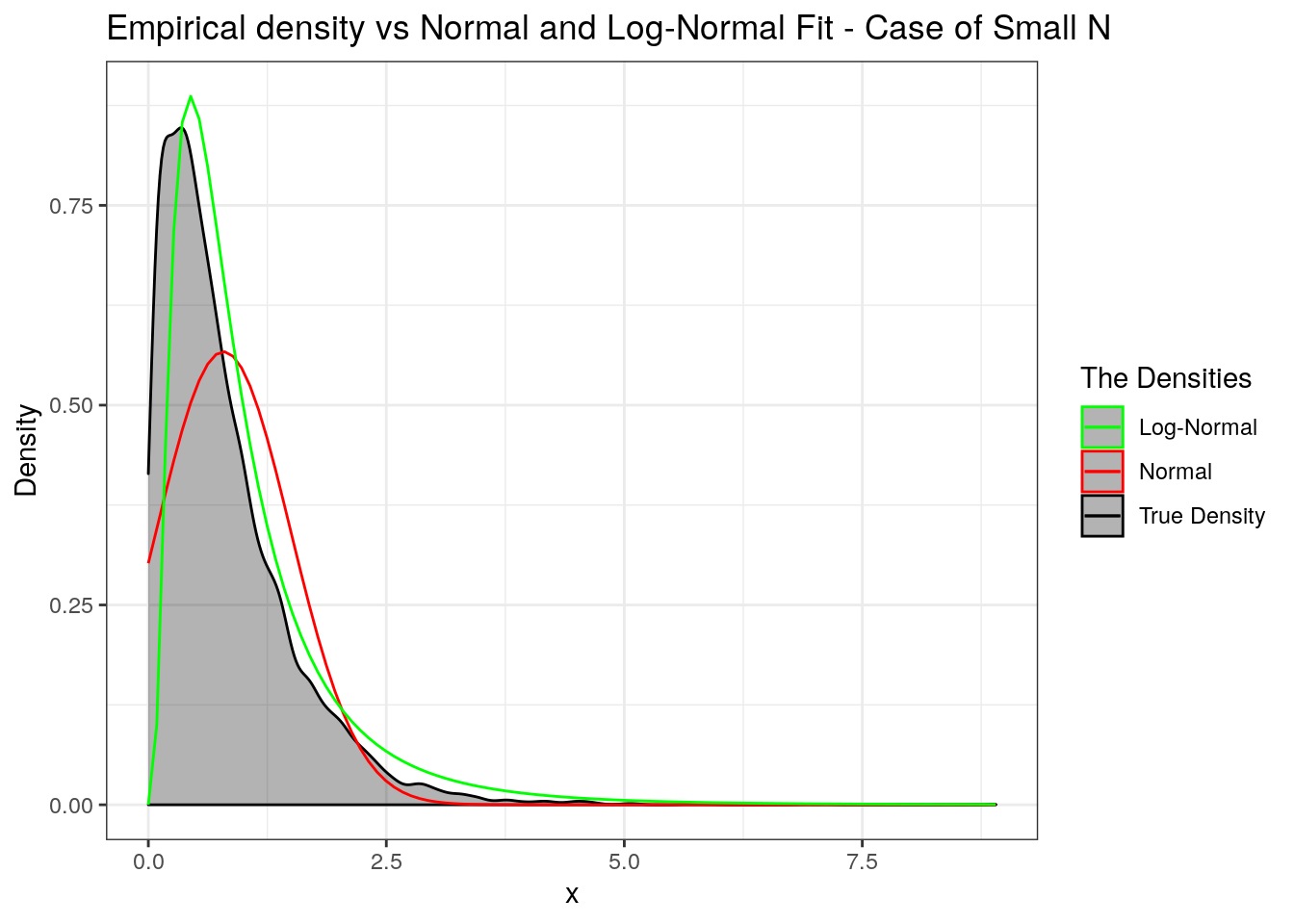
We will wrap up by repeating the same for the case when \(N\) takes large values. So we step up \(\lambda\) from \(3\) to \(50\). Try different values and report your observations on Piazza. Also, I worked with a heavy tailed Pareto, especially with \(\alpha=5\) (with infinite fourth moment).
options(warn=-1)
# Simulating S
lambda<-50;
pa<-1-exp(-lambda); # Probability of acceptance
ps<-0.75; # Probability of Simulating enough

N<-truncsim(10000,pa,ps,function(n){rpois(n,lambda)},0,Inf) # Checked above!!

cumsumN<-c(1,1+cumsum(N));
X<-cumsum(simPareto(sum(N)+1,alpha,theta))
Y<-X[cumsumN]
Y<-Y-c(0,Y[-length(Y)])
S<-Y[-1] # S contains the compound random variables....

popmean_S<-1/4*lambda/pa;
popvar_S<-5/48*lambda/pa + 1/16*((lambda^2+lambda)/pa -(lambda/pa)^2);

# The mu and sigma for lognormal fit
ln_sigma<-sqrt(log((popvar_S+popmean_S^2)/(popmean_S^2)));
ln_mu<-log(popmean_S)-(1/2)*ln_sigma^22;

# Plotting to verify the code/method
library(ggplot2)
theme_set(theme_bw());

plotdata <- data.frame(my_sample = S);


suppressWarnings(p <- ggplot(data = plotdata) +
  stat_density(aes(x = my_sample,colour="True Density"), fill = "black",alpha = 0.3) +
  stat_function(aes(colour="Normal"),fun = function(x){dnorm(x,popmean_S,(popvar_S)^(1/2))}) +
  stat_function(aes(colour="Log-Normal"),fun = function(x){dlnorm(x,ln_mu,ln_sigma)}) +
  labs(title = "Empirical density vs Normal and Log-Normal Fit - Case of Large N",
       x = "x", y = "Density") +
    scale_colour_manual("The Densities", values = c("green", "red", "black")))
p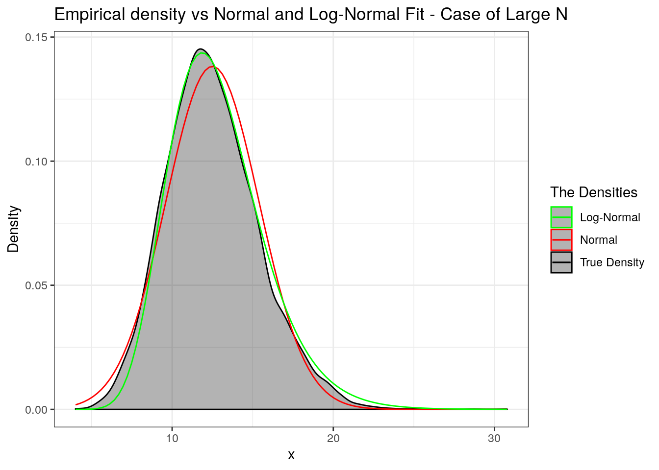
The upshot - If \(N\) assumes large values then the normal approximation is preferred but log-normal does well if \(X_i\)’s are heavy tailed. If \(N\) assumes small values then use the log-normal approximation.