6 Likelihood Ratio Based Confidence Regions
In this note I will give you some heuristics for the likelihood ratio based confidence region, and then show via simulation that it leads to better small sample performance compared to what we get using the asymptotic normality of the MLE.
6.1 Heuristics
Let \(l(\cdot)\) denote the loglikelihood, and let \(\tilde{\theta}\) denote the \(d\) dimensional parameter taking value in \(\Theta\subseteq \mathbb{R}^d\). We denote by \(\tilde{\theta}_0\) the true underlying parameter and by \(\hat{\theta}\) the MLE. Also, we assume that the MLE asymptotic normality holds, i.e.
\[
\sqrt{n}\left(\hat{\theta}-\theta_0\right)\buildrel {\rm d} \over \longrightarrow N_d\left(\tilde{0},\left(I(\tilde{\theta}_0)\right)^{-1}\right)
\]
where \(I(\cdot)\) is the information matrix and is given by
\[
I(\tilde{\theta})=\mathbb{E}{\left(\frac{\partial}{\partial \tilde{\theta}} f(X;\tilde{\theta})\frac{\partial}{\partial \tilde{\theta}} f(X;\tilde{\theta})^{\scriptscriptstyle\mathsf{T}}\right)}=-\mathbb{E}{\left(\frac{\partial^2}{\partial \tilde{\theta}^2} f(X;\tilde{\theta})\right)}.
\]
Now note that by using multivariate Taylor’s expansion we have,
\[
\begin{aligned}
l({\theta}_0) &\approx l(\hat{\theta}) + \dot{l}(\hat{\theta})^{\scriptscriptstyle\mathsf{T}} (\tilde{\theta}_0 - \hat{\theta}) + \frac{1}{2} (\tilde{\theta}_0 - \hat{\theta})^{\scriptscriptstyle\mathsf{T}} \ddot{l}(\hat{\theta}) (\tilde{\theta}_0 - \hat{\theta})\\
&=l(\hat{\theta}) + \frac{1}{2} (\tilde{\theta}_0 - \hat{\theta})^{\scriptscriptstyle\mathsf{T}} \ddot{l}(\hat{\theta}) (\tilde{\theta}_0 - \hat{\theta})
\end{aligned}
\]
In the above we denote the gradient and Hessian of \(l\) by \(\dot{l}\) and \(\ddot{l}\).
By using the consistency of the MLE, we have \(\hat{\theta}\buildrel {\rm d} \over \longrightarrow\tilde{\theta}_0\) this implies that
\[
(\tilde{\theta}_0 - \hat{\theta})^{\scriptscriptstyle\mathsf{T}} \ddot{l}(\hat{\theta}) (\tilde{\theta}_0 - \hat{\theta})=\sqrt{n}(\tilde{\theta}_0 - \hat{\theta})^{\scriptscriptstyle\mathsf{T}} \left(\frac{1}{n}\ddot{l}(\hat{\theta})\right) \sqrt{n}(\tilde{\theta}_0 - \hat{\theta})\approx \sqrt{n}(\tilde{\theta}_0 - \hat{\theta})^{\scriptscriptstyle\mathsf{T}} \left(\frac{1}{n}\ddot{l}(\tilde{\theta}_0)\right) \sqrt{n}(\tilde{\theta}_0 - \hat{\theta}).
\]
Now by using the LLN we have \(n^{-1}\ddot{l}(\tilde{\theta}_0)\buildrel {\rm d} \over \longrightarrow-I(\tilde{\theta}_0)\)
\[
\sqrt{n}(\tilde{\theta}_0 - \hat{\theta})^{\scriptscriptstyle\mathsf{T}} \left(\frac{1}{n}\ddot{l}(\tilde{\theta}_0)\right) \sqrt{n}(\tilde{\theta}_0 - \hat{\theta})
\approx -\sqrt{n}(\tilde{\theta}_0 - \hat{\theta})^{\scriptscriptstyle\mathsf{T}} I(\tilde{\theta}_0) \sqrt{n}(\tilde{\theta}_0 - \hat{\theta})
\]
Now note that if
\[Y\sim N_d\left(\tilde{0},\Sigma\right)\]
then
\[\Sigma^{-1/2}Y\sim N_d\left(\tilde{0},\Sigma^{-1/2}\Sigma\Sigma^{-1/2}\right)=N_d\left(\tilde{0},I_d\right).\]
In particular, we have
\[ \Sigma^{-1/2}Y^{\scriptscriptstyle\mathsf{T}} \Sigma^{-1/2}Y \sim \chi^2_d.\]
Combining this with the asymptotic normality of the MLE and the above observations, we have
\[
(\tilde{\theta}_0 - \hat{\theta})^{\scriptscriptstyle\mathsf{T}} \ddot{l}(\hat{\theta})(\tilde{\theta}_0 - \hat{\theta})\approx -\sqrt{n}(\tilde{\theta}_0 - \hat{\theta})^{\scriptscriptstyle\mathsf{T}} I(\tilde{\theta}_0) \sqrt{n}(\tilde{\theta}_0 - \hat{\theta}) \buildrel {\rm d} \over \longrightarrow-\chi^2_d
\]
Hence,
\[
\begin{aligned}
l({\theta}_0) &\approx l(\hat{\theta}) + \frac{1}{2} (\tilde{\theta}_0 - \hat{\theta})^{\scriptscriptstyle\mathsf{T}} \ddot{l}(\hat{\theta}) (\tilde{\theta}_0 - \hat{\theta})\\
&\approx l(\hat{\theta}) - \frac{1}{2} \chi^2_d.
\end{aligned}
\]
This suggests, that if we consider the region \(C_\alpha\subset\Theta\) defined by
\[
C_\alpha:=\left\{\tilde{\theta} : \frac{1}{2} \chi^2_{d:\alpha} \geq l(\hat{\theta}) - l({\theta}) \right\},
\]
where \(\chi^2_{d:\alpha}\) is the \(100(1-\alpha)\)-th percentile of \(\chi^2_{d}\), then the above implies that
\[
{\rm Pr}\left( \tilde{\theta}_0 \in C_\alpha \right)\rightarrow 1-\alpha.
\]
In other words, \(C_\alpha\) is an asymptotic \(100(1-\alpha)%\) confidence region for \(\tilde{\theta}\).
6.2 Why use the above?
Note that one could construct joint confidence regions a few different ways. One is to use asymptotic normal confidence intervals for each coordinate of \(\tilde{\theta}\) and using the Bonferroni method construct a hyper-rectangle with asymptotic level at least \(1-\alpha\). An improvement over this rudimentary idea is to use the following (Wald’s Confidence Region) suggested by the asymptotic normality of the MLE: \[ \left\{\tilde{\theta}: -(\tilde{\theta}- \hat{\theta})^{\scriptscriptstyle\mathsf{T}} \ddot{l}(\hat{\theta}) (\tilde{\theta} - \hat{\theta}) \leq \chi^2_{d,\alpha} \right\}. \] But how do we choose between two confidence regions? The likelihood ratio based region is clearly transformation (of the parameter) invariant while the Wald’s region is not and in fact choosing the right parametrization (aka transformation) may help. The other is that these are asymptotics justified regions - aka asymptotic confidence regions. The level of \((1-\alpha)\) hence is nominal - for small sample size the exact confidence level may differ. The method which yields a confidence region whose exact confidence level is closer to the nominal even for small sample sizes is naturally the preferred one. We will see below that the likelihood ratio based region fares better; this is so as the Wald’s method forces the region to be an ellipsoid centered at the MLE - which is inherently symmetric and is unable to accommodate the small sample skewness.
6.3 One Dimensional Example - Exponential
Consider an iid sample of size \(n\) from the exponential distribution with mean \(\theta\). In this case the 95% Wald’s confidence region is given by \[ \bar{x} \pm \frac{1.96 \bar{x}}{\sqrt{n}}, \] using the fact that the MLE of \(\theta\) is the mean and the variance of the exponential is given by \(\theta^2\). Below, we check the exact confidence level of this nominal 95% interval, and we note that the choice of \(\theta_0\) is irrelevant as \(\theta\) is a scale parameter and the interval is scale equivariant. Also I simulated 1,000,000 intervals as the standard error then equals \[ \frac{\sqrt{0.95*.05}}{1000}\approx 0.02%; \] so even \(3\times\)s.d. is less that 0.1%.
## theta_0=1
i<-1;
n_s<-100000;
s_vec<-c(5,10,15,25,50);
exact_level_1=rep(0,length(s_vec));
x<-matrix(rexp(max(s_vec)*n_s),ncol=max(s_vec))
for (n in s_vec){
  xbar<-apply(x[,1:n],1,mean);
  exact_level_1[i]<-sum((xbar-1.96*xbar/sqrt(n)<=1)&(xbar+1.96*xbar/sqrt(n)>=1))/n_s;
  i=i+1;
}
library("kableExtra")
results<-data.frame("Sample Size"=s_vec,"Exact Confidence Level"=round(100*exact_level_1,2));
results%>%
  kable(caption="Exact Confidence Level - Wald - Exponential") %>%
kable_styling(bootstrap_options = c("striped", "hover"),full_width=F,position="float_right") | Sample.Size | Exact.Confidence.Level |
|---|---|
| 5 | 86.92 |
| 10 | 90.28 |
| 15 | 91.81 |
| 25 | 92.98 |
| 50 | 94.01 |
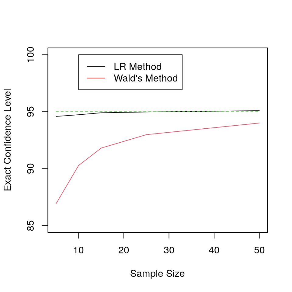
Now we do the same for the likelihood ratio based confidence region. It is easy to see that this region is given by (see Example 13.14 in the text if need be)
\[ \left\{ \theta: \frac{\bar{x}}{\theta}+\log(\theta) \leq 1+\log(\bar{x})+\frac{1.92}{n}\right\}. \] Now I will use a similar simulation setup as above to compute the exact confidence level of the likelihood ratio based confidence region (which happens to be an interval too - why?)
## theta_0=1
exact_level_2=rep(0,length(s_vec));
i<-1;
for (n in s_vec){
  xbar<-apply(x[,1:n],1,mean);
  exact_level_2[i]<-sum((xbar<=1+log(xbar)+1.92/n))/n_s;
  i=i+1;
}
plot(s_vec,100*exact_level_2,type="l",ylim=c(85,100),pch="*",ylab="Exact Confidence Level",xlab="Sample Size");
lines(s_vec,100*exact_level_1,pch="*",col=2);
lines(s_vec,rep(95,length(s_vec)),col=3,lty=2);
legend(10, 100, legend=c("LR Method", "Wald's Method"),
col=c("black", "red"),lty=rep(1,2))results<-data.frame("Sample Size"=s_vec,"Exact Confidence Level"=round(100*exact_level_2,2));
results%>%
kable(caption="Exact Confidence Level - Like. Ratio - Exponential") %>%
kable_styling(bootstrap_options = c("striped", "hover"),full_width=F,position="float_right") | Sample.Size | Exact.Confidence.Level |
|---|---|
| 5 | 94.58 |
| 10 | 94.73 |
| 15 | 94.90 |
| 25 | 94.97 |
| 50 | 95.09 |
To see the reason why the likelihood ratio confidence region does well, we for \(n=5\) construct the regions for \(\bar{x}\) equal to \(0.8,1\) and \(1.2\). Notice that while the Wald’s intervals are centered around the mean, the LR intervals are not.
f<-function(theta){return(xbar/theta+log(theta)-1-1.92/5-log(xbar))}
xbar=0.8;
x<-paste("(",round(uniroot(f,c(0.001,1))$root,3),",",round(uniroot(f,c(1,10))$root,3),")");
xbar=1;
y<-paste("(",round(uniroot(f,c(0.001,1))$root,3),",",round(uniroot(f,c(1,10))$root,3),")");
xbar=1.2;
z<-paste("(",round(uniroot(f,c(0.001,1))$root,3),",",round(uniroot(f,c(1,10))$root,3),")");
results<-data.frame("Mean"=c(0.8,1,1.2),"Wald\'s Interval"=c("(0.099,1.501)","(0.123,1.876)","(0.148,2.252)"),"LR Interval"=c(x,y,z));
library("kableExtra");
results%>%
  kable(caption="Wald and LR Confidence Intervals - n=5; Exponential with $\\theta=1$") %>%
kable_styling(bootstrap_options = c("striped", "hover"),full_width=F,position="float_right") | Mean | Wald.s.Interval | LR.Interval |
|---|---|---|
| 0.8 | (0.099,1.501) | ( 0.372 , 2.23 ) |
| 1.0 | (0.123,1.876) | ( 0.465 , 2.788 ) |
| 1.2 | (0.148,2.252) | ( 0.558 , 3.346 ) |
6.4 Two Dimensional Example - Gamma
Consider an iid sample of size \(n\) from a Gamma distribution with shape parameter \(\alpha\) and scale parameter \(\theta\) - note that mean equals \(\alpha\theta\). We first recall some observations from the previous note, and derive the asymptotic variance-covariance of the MLE. Just to fix the parametrization, the density is given by
\[ f_{\alpha,\theta}(x)=\frac{1}{\Gamma(\alpha)\theta^\alpha} e^{-(x/\theta)} x^{\alpha-1 },\quad x\geq 0; \] the parameter space is given by \((0,\infty)^2\).
6.4.1 Information Matrix
We note that, the log-likelihood is given by, \[ l(\alpha,\theta):=-n\log\Gamma(\alpha) - n\alpha\log\theta - \frac{1}{\theta}\sum_{i=1}^n x_i +(\alpha-1)\sum_{i=1}^n \log x_i. \] Now we observe that \[ \frac{\partial }{\partial \theta}l(\alpha,\theta) =-\frac{n\alpha}{\theta} +\frac{1}{\theta^2}\sum_{i=1}^n x_i, \] and \[ \frac{\partial^2 }{\partial \theta^2}l(\alpha,\theta) =\frac{n\alpha}{\theta^2} -\frac{2}{\theta^3}\sum_{i=1}^n x_i. \] In particular, the above yields \[ \mathbb{E}{\left(\frac{\partial^2 }{\partial \theta^2}l(\alpha,\theta)\right)} =\frac{n\alpha}{\theta^2} -\frac{2}{\theta^3}\mathbb{E}{\left(\sum_{i=1}^n X_i\right)}= \frac{n\alpha}{\theta^2} -\frac{2n\alpha\theta}{\theta^3}= -\frac{n\alpha}{\theta^2}. \] Also, we have \[ \frac{\partial^2 }{\partial \alpha \partial \theta}l(\alpha,\theta) =-\frac{n}{\theta}. \] On the other hand, \[ \frac{\partial }{\partial \alpha}l(\alpha,\theta) =-\frac{n\Gamma'(\alpha)}{\Gamma(\alpha)} + \sum_{i=1}^n \log x_i, \] and \[ \frac{\partial^2 }{\partial \alpha^2}l(\alpha,\theta) =n\left[\frac{\left(\Gamma'(\alpha)\right)^2}{\Gamma^2(\alpha)}-\frac{\Gamma''(\alpha)}{\Gamma(\alpha)}\right] \] Putting the above together gives us the information matrix
\[ I(\alpha,\theta)= \left(\begin{array}{cc} \left[\frac{\Gamma''(\alpha)}{\Gamma(\alpha)}-\frac{\left(\Gamma'(\alpha)\right)^2}{\Gamma^2(\alpha)}\right] & \frac{1}{\theta}\\ \frac{1}{\theta} & \frac{\alpha}{\theta^2} \end{array}\right) \]
6.4.2 The MLE
Recall from the previous note that \[ \hat{\theta}_{MLE}= \frac{\bar{x}}{\hat{\alpha}_{MLE}}. \] with \(\hat{\alpha}_{MLE}\) defined as \[ \arg \max_{\alpha} l(\alpha,\bar{x}/\alpha)=\arg \max_{\alpha}\left(-\log\Gamma(\alpha) - \alpha\log{\bar{x}}+ \alpha\log{\alpha} - \alpha + (\alpha-1)\frac{1}{n}\sum_{i=1}^n \log x_i\right), \] or equivalently as the root of \[ \log{\alpha} - \frac{\Gamma'(\alpha)}{\Gamma(\alpha)}=\log{\bar{x}} - \frac{1}{n}\sum_{i=1}^n \log x_i, \] where the lhs is a decreasing function of \(\alpha\) (see the previous note for its plot). In fact that it is decreasing can be inferred from the fact that \(I(\alpha,\theta)\) is positive semidefinite (Why? Think determinant!).
6.4.3 The Asymptotic Distribution of the MLE
With the sampling distribution taken to be a gamma with \(\alpha=3\) and \(\theta=2\), we simulate 1,000 samples of size \(10\), and for each sample we compute the MLEs of \(\alpha\) and \(\theta\). Then we estimate the bivariate kernel density estimate and compare it with the asymptotic distribution.
library(MASS);
# A function that returns the MLEs for a given data vector x
MLE_Gamma<-function(x){
  n<-length(x);
  rhs<-log(mean(x))-mean(log(x));
  like_der<-function(a){
    log(a)-digamma(a)-rhs
  }
  amle<-uniroot(like_der,interval=c(0.001,100))$root
  return(c(amle,mean(x)/amle))
}
n<-50;
n_sim<-1000;
mles<-t(apply(matrix(rgamma(n*n_sim,3,1/2),ncol=n),1,MLE_Gamma));
mles.kde <- kde2d(mles[,1], mles[,2], n=50);
# Simulating from the exact Asymptotic Normal
sim_true<-mvrnorm(100000,c(3,2),solve(rbind(c(trigamma(3),1/2),c(1/2,3/4)))/n);
sim_true.kde <- kde2d(sim_true[,1], sim_true[,2], n=50);
par(mfrow=c(1,2))
contour(mles.kde,xlim=c(0,6),col=1,ylim=c(0,4),main="Est. Joint Density of MLEs - n=50")
contour(sim_true.kde, col=2,xlim=c(0,6),ylim=c(0,4),main="Asymptotic Binormal Contours")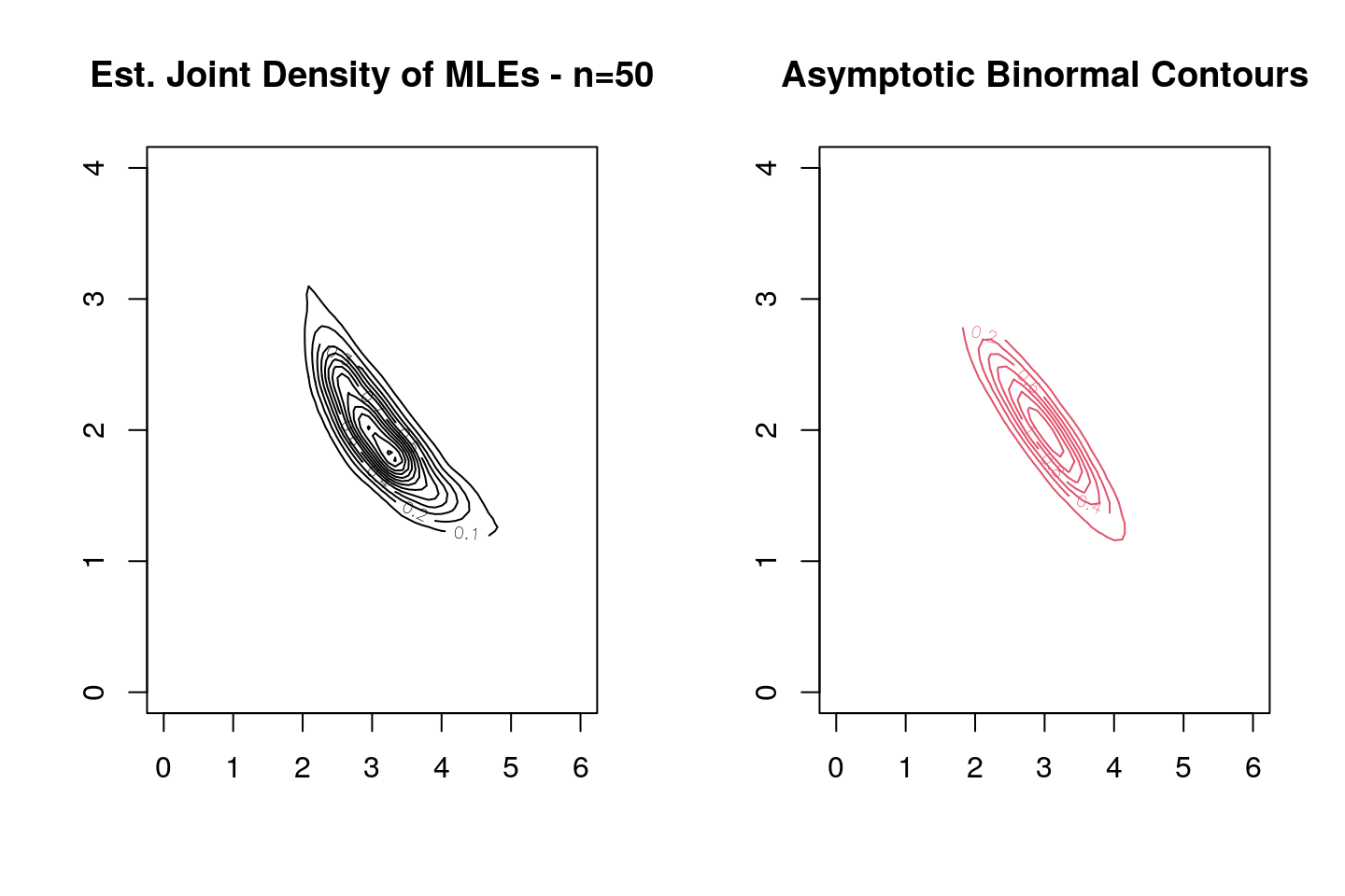
An alternate and prettier plot is found below. This was contributed by Sak Lee, a doctoral student in actuarial science at U. Iowa.
library(ggplot2)
library(cowplot)
library(latex2exp)
set.seed(76543)
generate_mles <- function(n, n_sim){
    sample_matrix <- matrix(rgamma(n * n_sim, shape = 3, scale = 2), ncol = n)
    mles <- t(apply(sample_matrix, 1, MLE_Gamma))
    data.frame(alpha = mles[,1],
               theta = mles[,2])
}

# Simulating from the exact Asymptotic Normal
generate_asymp <- function(n, n_sim){
    sim_true <- mvrnorm(n_sim,
                        c(3, 2), # mu vector
                        solve(rbind(c(trigamma(3),1/2), c(1/2,3/4)))/ n) # sigma
    data.frame(alpha = sim_true[,1],
               theta = sim_true[,2])
}

# Plotting
draw_2d_contour <- function(data_xy){
    ggplot(data = data_xy,
           aes(x = data_xy[,1], y = data_xy[,2])) +
        # Add points
        geom_point(fill = "gray",
                   size = 0.5,
                   alpha = 0.2) +
        # Add contour
        stat_density_2d(aes(fill = ..level..), geom = "polygon",
                        colour="white",
                        alpha = 0.7) +
        # Add Color and match with levels
        scale_fill_distiller(palette= "Spectral", direction=-1) +
        theme_bw()
}

plotdata1 <- generate_mles(50, 1000)
plotdata2 <- generate_asymp(50, 1000)

#Cowplot for multi plotting
p1 <- draw_2d_contour(plotdata1) +
        xlim(1, 6) +
        ylim(0, 4) +
        labs(title = paste("Est. Joint Density of MLEs - n=50"),
             x = TeX('$\\hat{\\alpha}$'),
             y = TeX('$\\hat{\\theta}$'))

p2 <- draw_2d_contour(plotdata2) +
        xlim(1, 6) +
        ylim(0, 4) +
        labs(title = paste("Asymptotic Binormal Contours"),
             x = TeX('$\\hat{\\alpha}$'),
             y = TeX('$\\hat{\\theta}$'))

plot_grid(p1, p2, ncol=2)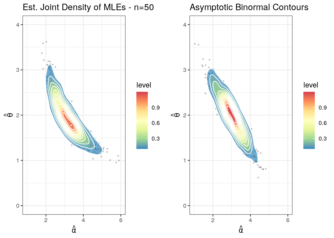
6.4.4 The Shape of the Three Confidence Regions
We will below plot the confidence regions derived using the methods of Bonferroni, Wald and the likelihood ratio. For this discussion we will fix the following sample of size \(50\), along with its MLEs and estimated information matrix.
set.seed(12345);
mle<-MLE_Gamma(x<-rgamma(50,3,1/2));
mle
## [1] 3.403929 2.187826est_inf_matrix<-rbind(c(trigamma(mle[1]),1/mle[2]),c(1/mle[2],mle[1]/mle[2]^2));
est_inf_matrix## [,1] [,2]
## [1,] 0.3410878 0.4570747
## [2,] 0.4570747 0.7111396inv_est_inf_matrix<-solve(est_inf_matrix);
inv_est_inf_matrix## [,1] [,2]
## [1,] 21.13733 -13.58571
## [2,] -13.58571 10.138216.4.4.1 Bonferroni Confidence Regions
The Bonferroni bounds use something called union bounds. So if \(C_\theta\) and \(C_\alpha\) are confidence regions for \(\theta\) and \(\alpha\) respectively, then
\[ {\rm Pr}\left(\theta_0\in C_\theta \cap \alpha_0\in C_\alpha\right)=1-{\rm Pr}\left(\theta_0\notin C_\theta \cup \alpha_0\notin C_\alpha\right) \geq 1-\left({\rm Pr}\left(\theta_0\notin C_\theta\right) + {\rm Pr}\left(\alpha_0\notin C_\alpha\right)\right). \]
In particular, if \(C_\theta\) and \(C_\alpha\) are 97.5% level confidence regions, then \(C_\alpha\times C_\alpha\) is a confidence region for \((\alpha,\theta)\) with level at least 95% - if \(C_\theta\) and \(C_\alpha\) are intervals, then we get a rectangle and in large dimensions hyperrectangles. For the above sample, this rectangle will be computed as follows:
l_a<-mle[1]-qnorm(0.9875)*sqrt(inv_est_inf_matrix[1,1]/50);
u_a<-mle[1]+qnorm(0.9875)*sqrt(inv_est_inf_matrix[1,1]/50);
l_t<-mle[2]-qnorm(0.9875)*sqrt(inv_est_inf_matrix[2,2]/50);
u_t<-mle[2]+qnorm(0.9875)*sqrt(inv_est_inf_matrix[2,2]/50);
(paste("(",round(l_a,3),",",round(u_a,3),")","x","(",round(l_t,3),",",round(u_t,3),")"))
## [1] "( 1.947 , 4.861 ) x ( 1.179 , 3.197 )"6.4.4.2 Wald’s Confidence Region
The Wald’s confidence region uses the asymptotic MLE to construct an elliptical confidence region. To see this, note that if \(\eta:=(\alpha,\theta)\), \(\eta_0:=(\alpha_0,\theta_0)\) then we have
\[
\sqrt{n}\left(\hat{\eta}-\eta_0\right)\buildrel {\rm d} \over \longrightarrow N_d\left(\tilde{0},\left(I(\alpha_0,\theta_0)\right)^{-1}\right).
\]
This and LLN implies that
\[
\sqrt{n}\left(\hat{\eta}-\eta_0\right)I(\hat{\alpha},\hat{\theta})\sqrt{n}\left(\hat{\eta}-\eta_0\right)^{\scriptscriptstyle\mathsf{T}} \approx \chi^2_{2}
\]
Hence, this suggests that
\[
\left\{\eta\left|\right. \sqrt{n}\left(\eta-\hat{\eta}\right)I(\hat{\alpha},\hat{\theta})\sqrt{n}\left(\eta-\hat{\eta}\right)^{\scriptscriptstyle\mathsf{T}}\leq \chi^2_{2;95\%} \right\},
\]
is an asymptotic 95% confidence region. The plot of this region for the above sample is found below.
6.4.4.3 Likelihood Ratio Based Confidence Region
# Bonferroni Rectangle
library(ellipse)
library(rootSolve)
plot(seq(l_a,u_a,length.out=100),rep(l_t,100),xlim=c(l_a-1,u_a+1),ylim=c(l_t-1,5),type="l",xlab=expression(hat(alpha)), ylab=expression(hat(theta)),main="The Three Confidence Regions");
lines(seq(l_a,u_a,length.out=100),rep(u_t,100));
lines(rep(l_a,100),seq(l_t,u_t,length.out=100));
lines(rep(u_a,100),seq(l_t,u_t,length.out=100));
# Wald's Confidence Region
lines(ellipse(inv_est_inf_matrix/50,centre=mle,level=0.95),col=2)
lines(mle[1],mle[2],type="p",col=3)
# LR Confidence Region
logx_bar<-mean(log(x));
x_bar<-mean(x);
rhs<--log(gamma(mle[1]))-mle[1]*log(x_bar)+mle[1]*log(mle[1])-mle[1]+(mle[1]-1)*logx_bar-qchisq(0.95,2)/(2*50);
# Range of Alpha Values
lalpha<-function(alpha){
  -log(gamma(alpha))-alpha*log(x_bar)+alpha*log(alpha)-alpha+(alpha-1)*logx_bar-rhs
}
range_alpha<-uniroot.all(lalpha,c(0.001,10))+c(0.001,-0.001)
# The Theta Values
theta_alpha<-function(alpha){
  f<-function(theta){
  -log(gamma(alpha))-alpha*log(theta)-x_bar/theta+(alpha-1)*logx_bar-rhs
  }
  uniroot.all(f,c(0.01,10))
}
# Plotting
theta<-matrix(unlist(sapply(seq(range_alpha[1],range_alpha[2],length.out=1000),theta_alpha)),nrow=1000,byrow=TRUE);
lines(c(seq(range_alpha[1],range_alpha[2],length.out=1000),seq(range_alpha[2],range_alpha[1],length.out=1000),range_alpha[1]),c(theta[,1],rev(theta[,2]),theta[1,1]),col=4);
# Legend
legend("topright",legend=c("MLE","Bonferroni", "Wald's Method","LR Method"),
       col=c("green","black", "red","blue"),lty=c(0,1,1,1),pch=c(1,NA,NA,NA),xpd=TRUE)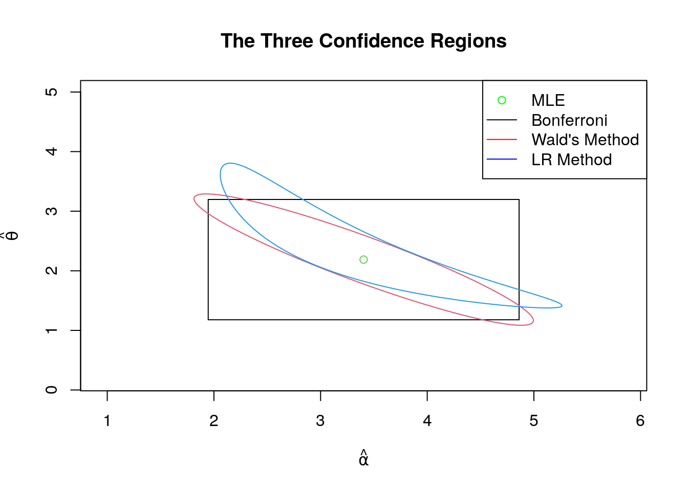
The Wald’s and LR confidence regions will align with increasing sample size (as the limit is bivariate normal and its contours are elliptical), but the Bonferroni will always be a rectangle. But as we show below, for small sample sizes the difference in shape matters!
6.4.5 Comparison of the Exact Confidence Levels
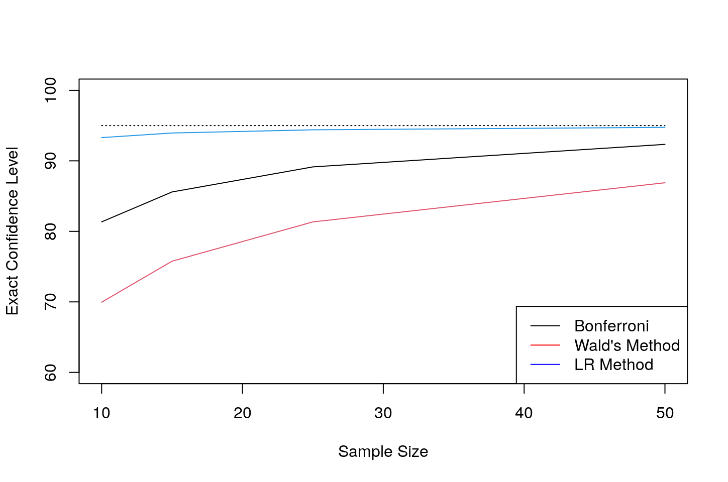
The below code computes the exact confidence level across various sample sizes. The sampling gamma distribution is as above. Note than the Bonferroni intervals do better on the exact confidence level, but note that they are much bigger in size that the other two - refer to the plot above.
set.seed(12345)
i<-1;
n_s<-100000;
s_vec<-c(10,15,25,50);
exact_level=matrix(rep(0,3*length(s_vec)),ncol=3);
x<-matrix(rgamma(max(s_vec)*n_s,shape=3,rate=1/2),ncol=max(s_vec))
exact<-function(z){ #c(alphamle,thetamle,n,truealpha,truetheta,xbar,logx_bar,)
    est_inf_matrix<-rbind(c(trigamma(z[1]),1/z[2]),c(1/z[2],z[1]/z[2]^2));
    inv_est_inf_matrix<-solve(est_inf_matrix);
    e<-rep(0,3);
    # Bonferroni
        l_a<-z[1]-qnorm(0.9875)*sqrt(inv_est_inf_matrix[1,1]/z[3]);
        u_a<-z[1]+qnorm(0.9875)*sqrt(inv_est_inf_matrix[1,1]/z[3]);
        l_t<-z[2]-qnorm(0.9875)*sqrt(inv_est_inf_matrix[2,2]/z[3]);
        u_t<-z[2]+qnorm(0.9875)*sqrt(inv_est_inf_matrix[2,2]/z[3]);
        e[1]<-(l_a<=z[4])&(l_t<=z[5])&(u_a>=z[4])&(u_t>=z[5]);
    # Wald's Method
        e[2]<-(z[3]*t(z[1:2]-z[4:5])%*%est_inf_matrix%*%(z[1:2]-z[4:5])<=qchisq(0.95,2));
    # LR Method
        rhs<--log(gamma(z[1]))-z[1]*log(z[6])+z[1]*log(z[1])-z[1]+(z[1]-1)*z[7]-qchisq(0.95,2)/(2*z[3]);
        e[3]<- (-log(gamma(z[4]))-z[4]*log(z[5])-z[6]/z[5]+(z[4]-1)*z[7]-rhs>=0);
    return(e);
}
# Various Sample Sizes
for (n in s_vec){
  mle<-t(apply(x[,1:n],1,MLE_Gamma));
  xbar<-apply(x[,1:n],1,mean);
  logx_bar<-apply(log(x[,1:n]),1,mean);
  z<-cbind(mle,rep(n,n_s),rep(3,n_s),rep(2,n_s),xbar,logx_bar);
  exact_level[i,]<-apply((apply(z,1,exact)),1,mean)
  i=i+1;
}
# Table
results<-data.frame("Sample Size"=s_vec,"Bonferroni"=round(100*exact_level[,1],2),"Wald\'s Method"=round(100*exact_level[,2],2),"LR Method"=round(100*exact_level[,3],2));
results%>%
  kable(caption="Exact Confidence Levels - Gamma(3,2)") %>%
kable_styling(bootstrap_options = c("striped", "hover"),full_width=F,position="float_right")| Sample.Size | Bonferroni | Wald.s.Method | LR.Method |
|---|---|---|---|
| 10 | 81.34 | 69.95 | 93.30 |
| 15 | 85.59 | 75.77 | 93.95 |
| 25 | 89.14 | 81.34 | 94.40 |
| 50 | 92.34 | 86.89 | 94.75 |
# Plot
plot(s_vec,100*exact_level[,1],type="l",ylim=c(60,100),col=1,pch="*",ylab="Exact Confidence Level",xlab="Sample Size");
lines(s_vec,100*exact_level[,2],pch="*",col=2);
lines(s_vec,100*exact_level[,3],pch="*",col=4);
lines(s_vec,rep(95,length(s_vec)),col=1,lty=3);
legend("bottomright", legend=c("Bonferroni","Wald's Method","LR Method"),
       col=c("black","red","blue"),lty=rep(1,2))