8 Parallel Computing in R
8.1 Introduction
You may have noticed that the top processor speeds have for the past decade or so stagnated around 4GHz - this is due to the implications of the underlying physics in terms of heat dissipation and power consumption. So how are we getting stuff done faster, you may ask. The answer is that while the clock speed of processors are not growing, the number of computing cores in the processors is growing. And a not-so-new programming paradigm called parallel programming is being employed to divide many jobs up into smaller pieces, and fully utilizing these cores leads to improved job execution times.
In the following I will walk you through doing some parallel programming on R and in the process learning to fully utilize your computer’s computing cores. And BTW, professional actuarial software like ALFA, GGY Axis, MoSes etc.. do subscribe to this paradigm, but they dumb it down so that actuaries can reap the benefits by just checking a few check boxes and pressing a button. So in the following you would also get a glimpse of what these softwares do under the hood.
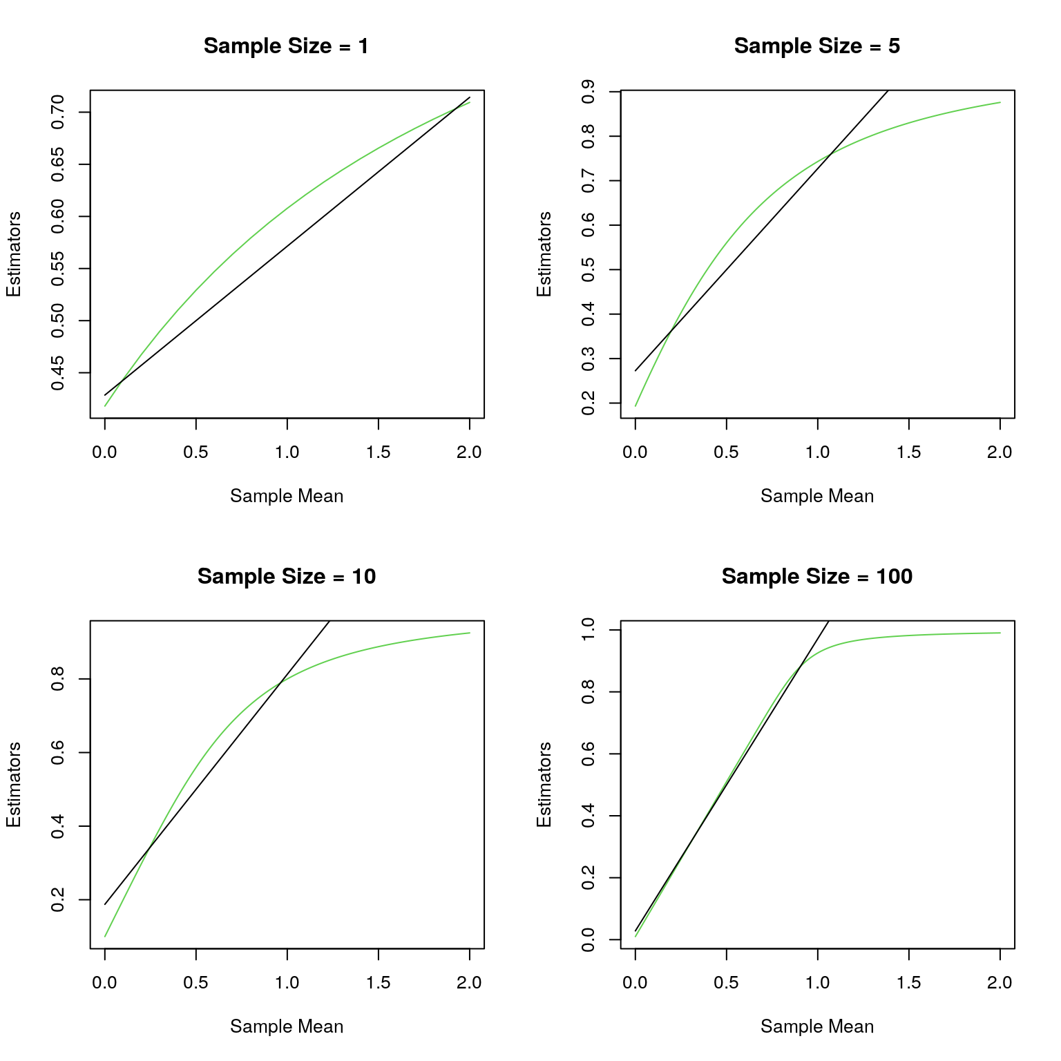
Description of the problem: Recall the credibility problem with Poisson counts with the Poisson mean being assigned the U(0,1) prior. I derived the Bayesian estimator for the Poisson mean as well as the Buhlmann credibility estimator. In this exercice we will compare how the Bayes estimator compares to the Buhlmann credibility estimator, especially in terms of mean-squared error and Bayes risk.
To warm up I will plot the two estimators as a function of the sample mean, which is a complete sufficent statistic.
set.seed("8464749")
Bayes_est<-function(s){ # The Bayes Estimator as a function of the sample sum
  ss<-1;
  for (k in 1:30){
    ss<-ss+n^k/prod(s+((k+1):2));
  }
  return((1-1/ss)*(s+1)/n)
}

par(mfrow=c(2,2));

for (n in c(1,5,10,100)) {
x<-(0:floor(20*n))/10;
plot(x/n,unlist(lapply(x,Bayes_est)),type="l",xlab="Sample Mean",ylab="Estimators",col=3,main=paste("Sample Size =",as.character(n)))
lines(x/n,(x+3)/(n+6),type="l") # Buhlmann Credibility Estimator
}
A simple workflow to compute in parallel on R is the following:
Step 1.: Start a pool of M workers where M \(\leq\) the number of cores that you have. First, we will invoke the library parallel and check the number of computing cores on our machines:
library(parallel);
library(emo);
library(doSNOW);
ncores<-detectCores();
ncores
## [1] 128The hpc server allows us to use 128 (logical) cores; note that the number of logical cores can be twice as much as the number of physical cores, made available through a technology which used to be called hyperthreading. So while I should expect at least a twelve-fold improvement on embarrassingly parallel jobs, one should know that sometimes hyperthreading can hurt. Also, sometimes we can see a slight improvement by using twice the number of process threads as the logical cores. Upshot: you need to experiment and find how many threads you want to use. In the problem above, hyperthreading is not of much help 😿 as the computational job is CPU-bound.
But not so impressive is the fact that I have not demonstrated to you yet how to makes use of this power. So here we go …
cl<-makeCluster(ncores<-24); # I am creating 24 worker processes or threads ... even though as we will see that I essentially get a four fold improvementStep 2.: Initialize the workers with libraries, function defns., data etc..
clusterEvalQ(cl,Bayes_est<-function(s){ # The Bayes Estimator as a function of the sample sum
  ss<-1;
  for (k in 1:30){
    ss<-ss+n^k/prod(s+((k+1):2));
  }
  return((1-1/ss)*(s+1)/n)
})
Step 3.: We now split the job among the worker processes, wait for them to complete their jobs, and collect their results. This step could be repeated many times in your program, as needed.
mse<-function(theta){
s<-rpois(100000,n*theta);
sqrt(n)*(mean(((s+3)/(n+6)-theta)^2)-mean((unlist(lapply(s,Bayes_est))-theta)^2))
}
theta<-(1:100)/100;
invisible(clusterEvalQ(cl,n<-5)); #data sent to all the workers; invisible used to suppress output
system.time(mse_vec<-unlist(parLapply(cl,theta,mse))); # Note that parLapply automatically send the defn. of mse to all the workers
## user system elapsed
## 0.209 0.218 197.756Just to compare, the time it takes with one core and simple lapply
system.time(mse_vec<-unlist(lapply(theta,mse))); # Simple lapply - one core## user system elapsed
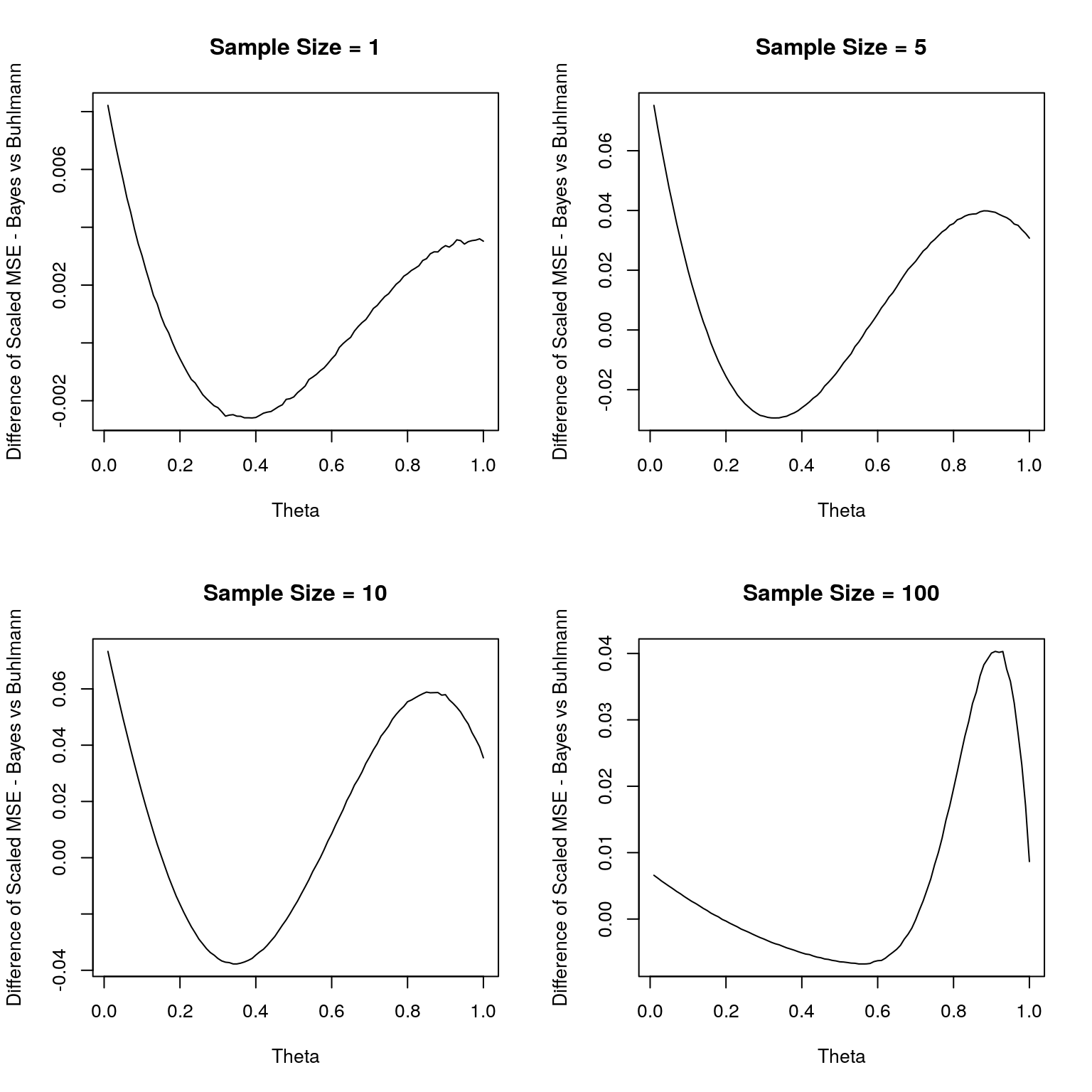
## 356.499 0.396 356.900Now, we will use parallel paradigm to compute the MSE of the Bayes and Buhlmann credibitlity estimators for varying sample sizes. Also, we use a simple approximation for the integral of the MSE in the interval (0,1) to approxmiate the difference in the Bayes risk.
par(mfrow=c(2,2));
i<-1;
diff_bayes_risk<-rep(0,4);
for (n in c(1,5,10,100)) {
invisible(clusterExport(cl,"n")); #data sent to all the workers; invisible used to suppress output
mse_vec<-unlist(parLapply(cl,theta,mse));
plot(theta,mse_vec,type="l",xlab="Theta",ylab="Difference of Scaled MSE - Bayes vs Buhlmann",col=1,main=paste("Sample Size =",as.character(n)));
diff_bayes_risk[i]<-mean(mse_vec[-1]);
i<-i+1;
}

par(mfrow=c(1,1));
plot(c(1,5,10,100),diff_bayes_risk,xlab="Sample Size",ylab="Diff. of Bayes Risk")
Step 4.: Shutdown the worker processes
stopCluster(cl)
registerDoSEQ()
The previous step is important to do so that we release the memory, and with that we have completed our first of the two parallel computing exercises. The second, deals with parallel computing with careful handling of the random number generation process, as will be explained below.
8.2 Random Number Generation
Note that when we do simulations an underlying assumption is that the primary set of simulated random variables are independent. And these are at the lowest level uniform (0,1) random numbers generated using some psuedo random number generator. All of the random generators that software use are periodic in nature; so one requirement for a good generator is that it has a large period. Also, we would require that if we form k-vectors by using the first k generated values, next k values, etc.. then these vectors are uniformly distributed in the k-dimensional unit cube. Interestingly, for some bad generators used in some software, with k=3 the vectors belonged to one of a set of 15 parallel planes in \(\mathbb{R}^3\) - very far from being uniform in the cube.
When we do simulations in parallel we need one more requirement: we should be able to guarantee that the random numbers generated by each worker process is independent of the other. While R’s default generator - Mersenne-Twister - is a very fine generator, it is not easy to offer the latter guarantee if one uses it. The scientific community largely employs the L’Ecuyer et al generator - L’Ecuyer. The generator is as follows:
\[ \begin{array}{rcl} x_n &=& 1403580x_{n-2} - 810728 x_{n-3} \mod (2^{32}-209)\\ y_n &=& 527612y_{n-1} - 1370589y_{n-3} \mod (2^{32}-22853)\\ z_n &=& (x_n-y_n) \mod 4294967087\\ u_n &=& z_n/4294967088 \hbox{ unless } z_n =0 \end{array} \] The seed consists of \((x_{n-3},x_{n-2},x_{n-1},y_{n-3},y_{n-2},y_{n-1})\), and what makes it preferable to the Mersenne-Twister is that we can advance the seed easliy and its seed is compact - only six integers. So let us see how we can use this:
set.seed(2018); # For reproducibility we start with a known seed
RNGkind(); # Check that the default generator is the Mersenne-Twister
## [1] "Mersenne-Twister" "Inversion" "Rejection"length(.Random.seed)-2; # The seed for the Mersenne-Twister is a set of 624 32-bit integers (The first number is an indentifier of the RNG and normal generator, and the second records the position in the 624 set )## [1] 624RNGkind("L'Ecuyer-CMRG"); # We now change the RNG to the L'Ecuyer RNG
RNGkind(); # Check that the default generator is the L'Ecuyer-CMRG## [1] "L'Ecuyer-CMRG" "Inversion" "Rejection"length(.Random.seed)-1; # The seed for the L'ecuyer et al RNG is only six integers (The first number is an indentifier of the RNG and normal generator)## [1] 6.Random.seed; # This is the current seed## [1] 10407 1688873339 1775859328 1151886465 -327940018 1168415863 -1120250292.Random.seed<-nextRNGStream(.Random.seed); # This advances the generator $2^{127}$ steps And this is what we need.
.Random.seed; # This is the advanced current seed## [1] 10407 -1216185839 -325430901 -551307425 1544164844 736709216 -829582134Now we are ready to do parallel simulations the right way:
ncores<-8;
cl<-makeCluster(ncores);
set.seed(23*89) # The first number of the form 2^p -1, for prime p, which is not a prime (Mersenne Prime) is 2047=23*89
RNGkind("L'Ecuyer-CMRG");
s<-.Random.seed;
for (i in (1:8)){
  invisible(clusterExport(cl[i],"s"));
  clusterEvalQ(cl[i],.Random.seed<-s);
  s<-nextRNGStream(s); # Advance by 2^127 steps
}
# Now we have set the streams in all of the workers to be independent - so we can proceed as usual
system.time(s<-mean(unlist(clusterEvalQ(cl,mean(rnorm(10000000))))))
## user system elapsed
## 0.002 0.000 2.953s## [1] -8.740055e-05stopCluster(cl);
registerDoSEQ();