Chapter Navigation

2.1 The List object 2.2 Working with an Aggregate Table 2.3 Table Retrieval and the various Data Fields of the List 2.4 Some Important Meta Data 2.5 Computing Actuarial Quantities

Chapter Navigation

2.1 The List object 2.2 Working with an Aggregate Table 2.3 Table Retrieval and the various Data Fields of the List 2.4 Some Important Meta Data 2.5 Computing Actuarial Quantities

2 Life Contingencies with R

The international section of the SOA (and the Technology section, I think!) through efforts over many years has collected the tables that are now available on the mort.soa.org. All of these tables are available in the Tables sub-directory of the shared class-notes directory in your rstudio.hpc server. So we assume your current working directory contains Tables folder, and the folder contains the files corresponding to all of the tables.

I wrote the two R function named mortalitytable and mortalitytableq that is available to you in the IntroR_Inc.R source file that you should simply source as shown below:

source("IntroR_Inc.R")

These will be useful to import mortality rates from tables that are available in the XML format on http://mort.soa.org.

2.1 The List object

There are many data structures in R, of which one of them is a list. The mortalitytable returns a list object which contains not only the mortality rates but also many meta data on the table. Below, I construct and populate a list object, and then show how to access/retrieve them. If need be, use R help or the internet to understand the following piece of code.

mylist<-list(name="Shyamal",
             num_children = 2,
             child_ages = c(14, 14),
             child_genders = c("Male","Female"),
             child_nationalities = matrix(c("Mexico","US","Mexico","US"),
                                          byrow=T, nrow=2));
mylist$name

## [1] "Shyamal"

mylist$num_children

## [1] 2

mylist$child_ages[2]

## [1] 14

mylist$child_nationalities[2,]

## [1] "Mexico" "US"

2.2 Working with an Aggregate Table

Below we will retrieve the 1980 Commissioners Standard Ordinary (CSO) Female. Basis: Age Last Birthday table, and derive some basic life contingencies quantities.

2.3 Table Retrieval and the various Data Fields of the List

mytab<-mortalitytable(35)
mytab

## $number
## [1] 35
## 
## $name
## [1] "1980 CSO – Female, ALB"
## 
## $layout
## [1] "Aggregate"
## 
## $usage
## [1] "CSO/CET"
## 
## $nation
## [1] "United States of America"
## 
## $select.minage
## [1] 0
## 
## $select.maxage
## [1] 99
## 
## $select.ageinc
## [1] 1
## 
## $select.mindur
## [1] 0
## 
## $select.maxdur
## [1] 100
## 
## $select.durinc
## [1] 1
## 
## $ult.minage
## [1] 0
## 
## $ult.maxage
## [1] 99
## 
## $ult.ageinc
## [1] 1
## 
## $qult
##   [1] 0.00188 0.00084 0.00080 0.00078 0.00077 0.00075 0.00073 0.00071 0.00070 0.00069
##  [11] 0.00068 0.00070 0.00073 0.00077 0.00082 0.00087 0.00092 0.00096 0.00100 0.00103
##  [21] 0.00106 0.00108 0.00110 0.00112 0.00115 0.00117 0.00120 0.00124 0.00128 0.00132
##  [31] 0.00137 0.00142 0.00147 0.00154 0.00161 0.00170 0.00182 0.00196 0.00213 0.00232
##  [41] 0.00253 0.00275 0.00298 0.00320 0.00344 0.00368 0.00392 0.00419 0.00448 0.00479
##  [51] 0.00513 0.00550 0.00592 0.00638 0.00685 0.00733 0.00780 0.00825 0.00870 0.00920
##  [61] 0.00980 0.01054 0.01149 0.01263 0.01392 0.01529 0.01671 0.01813 0.01959 0.02123
##  [71] 0.02316 0.02553 0.02847 0.03199 0.03605 0.04056 0.04545 0.05068 0.05632 0.06257
##  [81] 0.06967 0.07783 0.08725 0.09790 0.10962 0.12229 0.13582 0.15018 0.16538 0.18154
##  [91] 0.19885 0.21768 0.23869 0.26341 0.29523 0.34102 0.41388 0.53724 0.74396 1.00000

2.4 Some Important Meta Data

Is it aggregate?

mytab$layout

## [1] "Aggregate"

When Aggregate, what is the range of the ages, and is it quinquennial or annual table?

mytab$ult.minage

## [1] 0

mytab$ult.maxage

## [1] 99

mytab$ult.ageinc # To make sure it is annual and not quinquennial

## [1] 1

Retrieving all the Mortality Rates

q<-mytab$qult
q

##   [1] 0.00188 0.00084 0.00080 0.00078 0.00077 0.00075 0.00073 0.00071 0.00070 0.00069
##  [11] 0.00068 0.00070 0.00073 0.00077 0.00082 0.00087 0.00092 0.00096 0.00100 0.00103
##  [21] 0.00106 0.00108 0.00110 0.00112 0.00115 0.00117 0.00120 0.00124 0.00128 0.00132
##  [31] 0.00137 0.00142 0.00147 0.00154 0.00161 0.00170 0.00182 0.00196 0.00213 0.00232
##  [41] 0.00253 0.00275 0.00298 0.00320 0.00344 0.00368 0.00392 0.00419 0.00448 0.00479
##  [51] 0.00513 0.00550 0.00592 0.00638 0.00685 0.00733 0.00780 0.00825 0.00870 0.00920
##  [61] 0.00980 0.01054 0.01149 0.01263 0.01392 0.01529 0.01671 0.01813 0.01959 0.02123
##  [71] 0.02316 0.02553 0.02847 0.03199 0.03605 0.04056 0.04545 0.05068 0.05632 0.06257
##  [81] 0.06967 0.07783 0.08725 0.09790 0.10962 0.12229 0.13582 0.15018 0.16538 0.18154
##  [91] 0.19885 0.21768 0.23869 0.26341 0.29523 0.34102 0.41388 0.53724 0.74396 1.00000

Important Check: It is important to check that the last value in the mortality rates is 1, as otherwise the resulting distribution will have mass less than \(1\).

q[length(q)]

## [1] 1

How to extract the rates for \((65)\)?

# Method 1 - Brute force
q<-mytab$qult;
q_65<-q[(65+1-mytab$ult.minage):length(q)];
q_65

##  [1] 0.01529 0.01671 0.01813 0.01959 0.02123 0.02316 0.02553 0.02847 0.03199 0.03605
## [11] 0.04056 0.04545 0.05068 0.05632 0.06257 0.06967 0.07783 0.08725 0.09790 0.10962
## [21] 0.12229 0.13582 0.15018 0.16538 0.18154 0.19885 0.21768 0.23869 0.26341 0.29523
## [31] 0.34102 0.41388 0.53724 0.74396 1.00000

#Method 2 - mortalitytableq
mortalitytableq(mytab,65,0)

##  [1] 0.01529 0.01671 0.01813 0.01959 0.02123 0.02316 0.02553 0.02847 0.03199 0.03605
## [11] 0.04056 0.04545 0.05068 0.05632 0.06257 0.06967 0.07783 0.08725 0.09790 0.10962
## [21] 0.12229 0.13582 0.15018 0.16538 0.18154 0.19885 0.21768 0.23869 0.26341 0.29523
## [31] 0.34102 0.41388 0.53724 0.74396 1.00000

2.5 Computing Actuarial Quantities

First, we compute the curtate future lifetime corresponding to the above mortality table.

Method 1: Without using recurrence (Figure out why this works!)

p <- 1 - q;
kp0<-c(1,cumprod(p));
len_kp0<-length(kp0);
ex_1<-rev(cumsum(rev(kp0[-1])))/kp0[-len_kp0]

Method 2 (Recurrence): Using standard recurrence

ex_2<-rep(0,mytab$ult.maxage-mytab$ult.minage+1);
for (i in (mytab$ult.maxage-mytab$ult.minage):1) {
ex_2[i]<-p[i]*(ex_2[i+1]+1);
}
ex_1[1]

## [1] 74.94063

ex_2[1]

## [1] 74.94063

Check

Checking The Two Methods

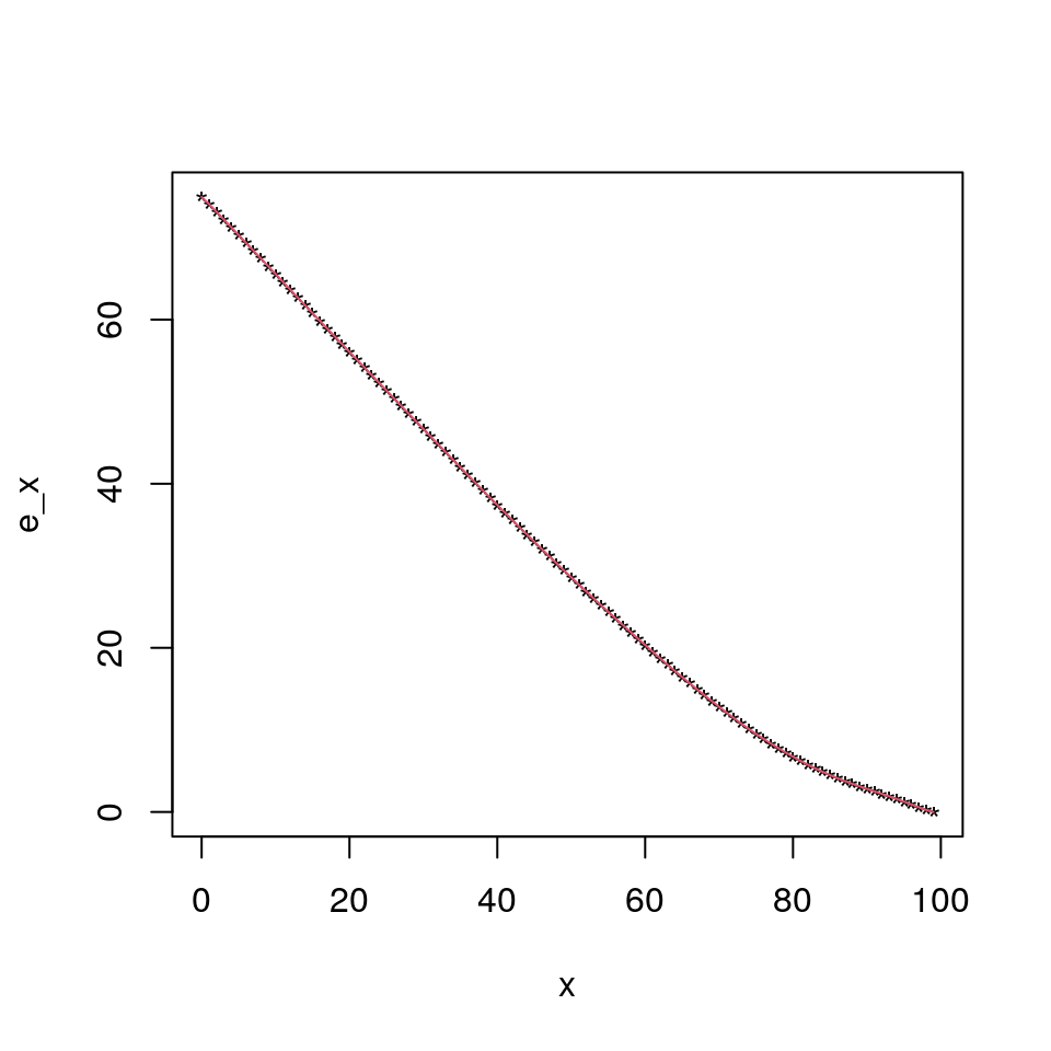
plot(0:(mytab$ult.maxage),ex_1,pch="*",ylab="e_x",xlab="x");
lines(0:(mytab$ult.maxage),ex_2,col=2);

Note that for complete future lifetime under UDD you can slap a \(0.5\) to the ex’s above. Or if you wish, you could do the following:

exc<-rep(0.5,mytab$ult.maxage-mytab$ult.minage+1); # Why did I use 0.5 here?
for (i in (mytab$ult.maxage-mytab$ult.minage):1) {
exc[i]<-p[i]*(exc[i+1]+1)+(1-p[i])*0.5;
}
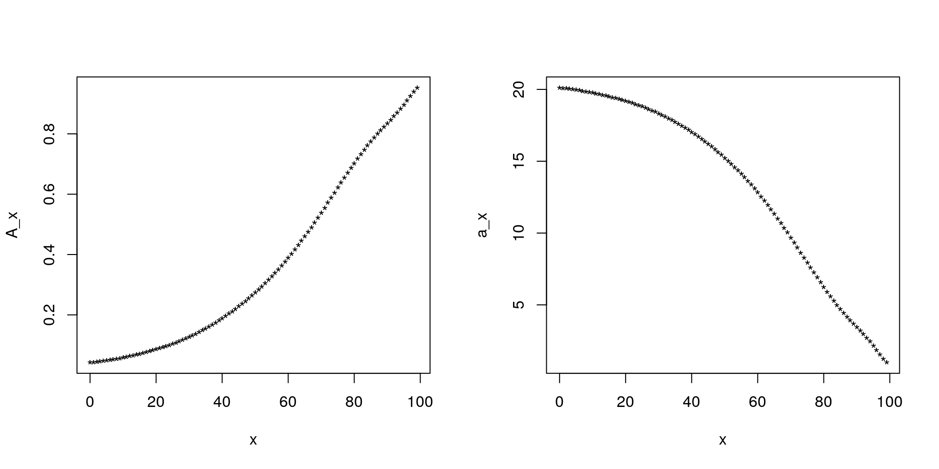
exc[1]-ex_1[1]-0.5

## [1] -4.263256e-14

Finally, here is how we can compute \(A_x\) and \(\ddot{a}_x\) for \(i=5\%\) :

v<-1/1.05;
Ax<-rep(v,mytab$ult.maxage-mytab$ult.minage+1); # Why did I use 0.5 here?
for (i in (mytab$ult.maxage-mytab$ult.minage):1) {
Ax[i]<-v*(p[i]*Ax[i+1]+(1-p[i]));
}

ax<-rep(1,mytab$ult.maxage-mytab$ult.minage+1); # Why did I use 1 here?
for (i in (mytab$ult.maxage-mytab$ult.minage):1) {
ax[i]<-v*p[i]*ax[i+1]+1;
}
mean((1-v)*ax+Ax) # Why should I get 1?

## [1] 1

par(mfrow=c(1,2));
plot(0:(mytab$ult.maxage),Ax,pch="*",ylab="A_x",xlab="x");
plot(0:(mytab$ult.maxage),ax,pch="*",ylab="a_x",xlab="x");

Whole Life Annuity and Insurance