10.1 Univariate Normal

Univariate normal is a central distribution in probability theory, and one reason for it is the Central Limit Theorem. Density of its standard version - with zero mean and unit variance - is given by \[ \frac{1}{\sqrt{2\pi}} \exp\left\{-x^2/2\right\}, \quad x\in \mathbb{R}. \] We denote this distribution by \(N(0,1)\), and using scaling and shifting we define the version with mean \(\mu\) and variance \(\sigma^2\). This is denoted by \(N(\mu,\sigma^2)\) and its density is easily seen to be \[ \frac{1}{\sqrt{2\pi}\sigma} \exp\left\{-(x-\mu)^2/(2\sigma^2)\right\}, \quad x\in \mathbb{R}. \] The moment generation function (mgf) of \(N(0,1)\) is easily derived using completion of squares, but it is fun to derive it as the limiting mgf of a standardized binomial random variable with parameters \(n\) and \(p\) as \(n\) approaches infinity- just do it ! The mgf of \(N(\mu,\sigma^2)\) is seen by either of the above two methods to be \[ \phi(t)=\exp\left\{\mu t + \sigma^2 t^2/2\right\}. \]

10.2 Multivariate Normal from Univariate Normal

Clearly, when we think of \(d\)-variate multivariate normal, we think of a joint density with normal marginals. So let us start with \(\widetilde{X}\) whose elements are \(d\) independent standard normal variates - denoted by \(N_d(\tilde{0},I_{d\times d})\). The notation will be seen to be valid shortly. As the mgf of \(\widetilde{X}\) equals \(\mathbb{E}{\left(\exp\{\tilde{t}'\widetilde{X}\}\right)}\), we have \[ \phi(\tilde{t}) = \exp\{\tilde{t}'\tilde{t}/2\}. \] Let \(d\times d\) matrix \(A\) be a non-singular matrix. Then \(\widetilde{Y}=\tilde{\mu}+A\widetilde{X}\) has mean \(\tilde{\mu}\), covariance matrix \(\Sigma\) given by \[ \Sigma=\mathbb{E}{\left(A\widetilde{X}\widetilde{X}'A'\right)}=A\mathbb{E}{\left(\widetilde{X}\widetilde{X}'\right)}A'=AA', \] mgf as
\[ \mathbb{E}{\left(\tilde{t}'\tilde{\mu}+\exp\{\tilde{t}'A\widetilde{X}\}\right)}=\mathbb{E}{\left(\exp\{\tilde{t}'\tilde{\mu}+(A'\tilde{t})'\widetilde{X}\}\right)}=\exp\{\tilde{t}'\tilde{\mu}+(A'\tilde{t})'A'\tilde{t}/2\}=\exp\{\tilde{t}'\tilde{\mu}+\tilde{t}'\Sigma\tilde{t}/2\}, \] and joint density given by \[ \frac{|A^{-1}|}{(\sqrt{2\pi})^d} \exp\left\{-(\tilde{y}-\tilde{\mu})'({A^{-1}})'A^{-1}(\tilde{y}-\tilde{\mu})/2\right\}=\frac{1}{(\sqrt{2\pi})^d|\Sigma|^{1/2}} \exp\left\{-(\tilde{y}-\tilde{\mu})'\Sigma^{-1}(\tilde{y}-\tilde{\mu})/2\right\}, \quad \tilde{y}\in \mathbb{R}^d. \] This distribution is defined as the \(d\)- dimensional multivariate normal with mean \(\tilde{\mu}\), covariance matrix \(\Sigma\), and denoted by \(N_d(\tilde{\mu},\Sigma)\).

10.3 Non-Multivariate-Normal with Normal Marginals

We first note that marginals being normals does not guarantee that the join distribution is multivariate normal. This is the first such bivariate example I encountered (in my sophomore year) - in Hogg and Craig: \[ \frac{1}{2\pi} \exp\{-(x_1^2+x_2^2)/2\}\left(1+x_1x_2\exp\left\{-(x_1^2+x_2^2-2)/2\right\}\right). \] The reason the marginals are standard normals is because the additional term is odd in \(x_1\) and \(x_2\), and the parenthetic term is non-negative (Why?).

Of course, there are many such examples - though the joint density are not as simply given as above. They can be constructed as follows: Take any \((X_1,X_2)\) following a continuous joint distribution with marginal cdfs \(F_1\) and \(F_2\). \(({F_1}(X_1),{F_2}(X_2))\) has uniform marginals, and hence \(({\Phi}^{-1}(F_1(X_1)),{\Phi}^{-1}(F_2(X_2))\) has standard normal marginals (\(\Phi\) is the cdf of \(N(0,1)\)). But clearly the generality implies that not all joints with normal marginals are multivariate normals. An instructive exercise will be to take a bivariate joint distribution of your choice, simulate from it and transform the simulated vectors to those with standard normal marginals, and check if the fitted joint density contours are elliptical.

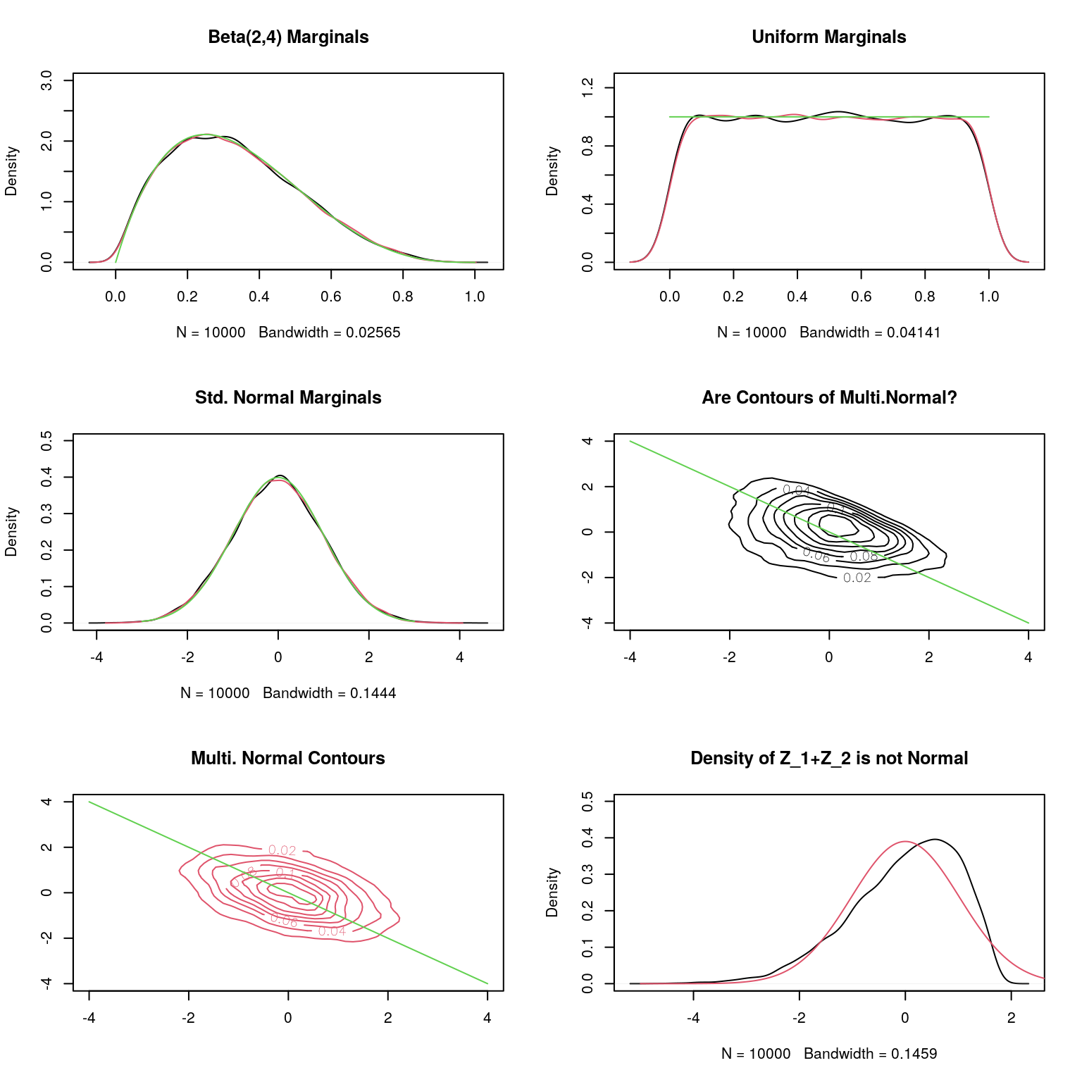
An interesting problem - can you design a simulation algorithm to simulate from the bivariate density above from Hogg and Craig?

10.4 Characterizing Property

Above we saw that in the case of our non-normal joint density that a linear function of the variables has a univariate non-normal distribution. Interestingly, if all of the linear functions of \(\widetilde{X}\) have a univariate normal density - let us call this property (L) - then the joint is a multivariate normal. To see this, note that (L) implies that there exists a \(\tilde{\mu}\) and \(\Sigma\) which satisfy (Why?) \[ \mathbb{E}{\left(\widetilde{X}\right)}=\tilde{\mu}, \hbox{and} \quad \Sigma=\mathbb{E}{\left(\widetilde{X}(\widetilde{X})'\right)}. \] Moreover, by (L) we also have \[ \mathbb{E}{\left(\exp\{\tilde{t}'\widetilde{X}\}\right)}=\exp\left\{\tilde{t}'\mu + \tilde{t}'\Sigma\tilde{t}/2\right\}, \] as \(\tilde{t}'\widetilde{X}\) has a univariate normal distribution with mean \(\tilde{t}'\mu\), and variance \(\tilde{t}'\Sigma\tilde{t}\). But the above is the mgf of \(\widetilde{X}\), and hence it follows a multivariate normal distribution.

10.5 Conditional Distribution

In the following \(\widetilde{X}\) is a random vector following \(N_d(\tilde{\mu},\Sigma)\), for a positive definite \(\Sigma\) - singular \(\Sigma\) can be reduced to the positive definite case. Also, we will partition \(\widetilde{X}\) as \(\widetilde{X}=(\widetilde{X}_1,\widetilde{X}_2)\), \(\tilde{\mu}\) as \(\tilde{\mu}=(\tilde{\mu}_1,\tilde{\mu}_2)\), and \(\Sigma\) as \[ \Sigma=\left(\begin{array}{cc} \Sigma_{11} & \Sigma_{12}\\ \Sigma_{21} & \Sigma_{22} \end{array}\right). \] It is easily seen from the mgf that the above partition (suitably defined) satisfies \(\widetilde{X}_i\sim N_{d_i}(\tilde{\mu}_i,\Sigma_{ii})\), for \(i=1,2\) (note \(d_1+d_2=d\)). Also, note that if \(\Sigma_{12}=O\), then the mgf can be factorized into the mgf of \(\widetilde{X}_1\) and \(\widetilde{X}_2\) and hence uncorrelated is equivalent to independence.

What we seek is the conditional distribution of \(\widetilde{X}_1\) given \(\widetilde{X}_2\) - we will use independence to get a slick derivation. Using an argument similar to one above, it is seen that \(A_{d\times d}\widetilde{X}\), for non-singular \(A\) - follows a multivariate normal distribution as well with positive definite covariance matrix \(A\Sigma A'\), and mean \(A\tilde{\mu}\). The idea is that if \(A\) of the form \[ A=\left(\begin{array}{cc} I & A_{12}\\ O & I \end{array}\right), \] can result in a diagonal \(A\Sigma A'\), then \(\widetilde{X}_1+A_{12}\widetilde{X}_2\) would be independent \(\widetilde{X}_{2}\). But that requires, \[ {\rm Cov}\left(\widetilde{X}_1+A_{12}\widetilde{X}_2,\widetilde{X}_{2}\right)=\Sigma_{12}+A_{12}\Sigma_{22}=O \quad \iff \quad A_{12}=-\Sigma_{12}\Sigma_{22}^{-1}. \] ence, we have \(\widetilde{X}_1-\Sigma_{12}\Sigma_{22}^{-1}\widetilde{X}_2\) is independent of \(\widetilde{X}_2\), and the former has a \(N_{d_1}(\tilde{\mu}_1-\Sigma_{12}\Sigma_{22}^{-1}\tilde{\mu}_2,\Sigma_{11}-\Sigma_{12}\Sigma_{22}^{-1}\Sigma_{21})\). The covariance matrix is derived as follows: \[ \begin{align*} \mathbb{E}{\left(\widetilde{X}_1-\Sigma_{12}\Sigma_{22}^{-1}\widetilde{X}_2(\widetilde{X}_1-\Sigma_{12}\Sigma_{22}^{-1}\widetilde{X}_2)'\right)}&=\mathbb{E}{\left(\widetilde{X}_1\widetilde{X}_1'\right)}+\mathbb{E}{\left(\Sigma_{12}\Sigma_{22}^{-1}\widetilde{X}_2\widetilde{X}_2'\Sigma_{22}^{-1}\Sigma_{21}\right)}\\ &\quad - \mathbb{E}{\left(\widetilde{X}_1\widetilde{X}_2'\Sigma_{22}^{-1}\Sigma_{21}\right)}-\mathbb{E}{\left(\Sigma_{12}\Sigma_{22}^{-1}\widetilde{X}_2\widetilde{X}_1'\right)}\\ &=\Sigma_{11}+\Sigma_{12}\Sigma_{22}^{-1}\Sigma{21}-\Sigma_{12}\Sigma_{22}^{-1}\Sigma{21}-\Sigma_{12}\Sigma_{22}^{-1}\Sigma{21}\\ &=\Sigma_{11}-\Sigma_{12}\Sigma_{22}^{-1}\Sigma_{21}. \end{align*} \] Now, by independence we have the conditional distribution of \(\widetilde{X}_1-\Sigma_{12}\Sigma_{22}^{-1}\widetilde{X}_2\) given \(\widetilde{X}_2\) is same as the unconditional distribution \(N_{d_1}(\tilde{\mu}_1-\Sigma_{12}\Sigma_{22}^{-1}\tilde{\mu}_2,\Sigma_{11}-\Sigma_{12}\Sigma_{22}^{-1}\Sigma_{21})\). But the conditional distribution of \(\widetilde{X}_1\) given \(\widetilde{X}_2\) is \(\Sigma_{12}\Sigma_{22}^{-1}\widetilde{X}_2\) shift of \(N_{d_1}(\tilde{\mu}_1-\Sigma_{12}\Sigma_{22}^{-1}\tilde{\mu}_2,\Sigma_{11}-\Sigma_{12}\Sigma_{22}^{-1}\Sigma_{21})\), i.e. \(N_{d_1}(\tilde{\mu}_1+\Sigma_{12}\Sigma_{22}^{-1}(\widetilde{X}_{2}-\tilde{\mu}_2),\Sigma_{11}-\Sigma_{12}\Sigma_{22}^{-1}\Sigma_{21})\). This is so as \[ \begin{aligned} \mathcal{L}(\widetilde{X}_1|\widetilde{X}_2)&=\mathcal{L}(\widetilde{X}_1-\Sigma_{12}\Sigma_{22}^{-1}\widetilde{X}_2+\Sigma_{12}\Sigma_{22}^{-1}\widetilde{X}_2|\widetilde{X}_2)\\ &=\mathcal{L}(\widetilde{X}_1-\Sigma_{12}\Sigma_{22}^{-1}\widetilde{X}_2|\widetilde{X}_2) \hbox{ shifted by } \Sigma_{12}\Sigma_{22}^{-1}\widetilde{X}_2\\ &= N_{d_1}(\tilde{\mu}_1-\Sigma_{12}\Sigma_{22}^{-1}\tilde{\mu}_2,\Sigma_{11}-\Sigma_{12}\Sigma_{22}^{-1}\Sigma_{21}) \hbox{ shifted by } \Sigma_{12}\Sigma_{22}^{-1}\widetilde{X}_2\\ &= N_{d_1}(\tilde{\mu}_1+\Sigma_{12}\Sigma_{22}^{-1}(\widetilde{X}_{2}-\tilde{\mu}_2),\Sigma_{11}-\Sigma_{12}\Sigma_{22}^{-1}\Sigma_{21}) \end{aligned} \]

10.6 Demonstrating Sufficiency - Normal Setting

Let us consider an \(n\)-sample from \(N(\mu,1)\) - \(\mu\) unknown. In the following we show that by compressing data to the sample mean, there is no loss of information with respect to the unknown \(\mu\).

We denote the original data by \(\widetilde{X}\), whose sample mean is denoted by \(\bar{X}\). We will be using \(\bar{X}\) to simulate \(\widetilde{Z}\) such that \[ \widetilde{Z} \buildrel \rm d \over =\widetilde{X}\sim N_d(\mu\mathbf{1},I_{d\times d}), \] thus establishing that the compression of the data to the sample mean in the normal setting is lossless.

Towards this, we define \(\widetilde{Y}\) such that \[ \widetilde{Y}=(X_1-\bar{X},\ldots,X_{d-1}-\bar{X},\bar{X}), \; \hbox{ with } A \hbox{ satisfying }\widetilde{Y}=A\widetilde{X}, \] and hence from the above we have, \[ \widetilde{Y}\sim N_d(\mu A\mathbf{1},AA'). \] For \(n=3\), the \(A\) matrix is given by \[ A=\left(\begin{array}{ccc} 2/3 & -1/3 & -1/3\\ -1/3 & 2/3 & -1/3\\ 1/3 & 1/3 & 1/3 \end{array}\right), \] and hence, \[ \widetilde{Y}\sim N_3\left(\left( \begin{array}{c} 0 \\ 0 \\ \mu \end{array}\right),\left(\begin{array}{ccc} 2/3 & -1/3 & 0\\ -1/3 & 2/3 & 0\\ 0 & 0 & 1/3 \end{array}\right)\right). \] Hence, we conclude that \[ \widetilde{Y}_{1:2}=(X_1-\bar{X},\ldots,X_{d-1}-\bar{X}) \hbox{ is independent of } \bar{X}, \] and follows \[ N_2\left(\left( \begin{array}{c} 0 \\ 0 \end{array}\right),\left(\begin{array}{cc} 2/3 & -1/3 \\ -1/3 & 2/3 \end{array}\right)\right), \] a distribution free of \(\mu\). Moreover, if we define \(\widetilde{Z}\) such that \[ \widetilde{Z}=\bar{X}\mathbf{1}+\left(\begin{array}{cc} 1 & 0 \\ 0 & 1\\ -1 & -1 \\ \end{array}\right)\widetilde{V}, \; \hbox{with } \widetilde{V}\sim N_2\left(\left( \begin{array}{c} 0 \\ 0 \end{array}\right),\left(\begin{array}{cc} 2/3 & -1/3 \\ -1/3 & 2/3 \end{array}\right)\right), \] and \(V\) independent of \(\bar{X}\) then \(\widetilde{Z}\buildrel \rm d \over =\widetilde{X}\). This is so as \[ (\bar{X},\widetilde{V})\buildrel \rm d \over =(\bar{X},\widetilde{Y}_{1:2}), \hbox{ and } \widetilde{Z}=\bar{X}\mathbf{1}+\left(\begin{array}{cc} 1 & 0 \\ 0 & 1\\ -1 & -1 \\ \end{array}\right)\widetilde{Y}_{1:2}. \] In the following we implement the simulation of \(\widetilde{Z}\).