11 Simulating Brownian Motion and Brownian Bridge
In this note I will introduce two stochastic processes, namely the Brownian Motion and the Brownian Bridge, show you how to simulate them, show how they are connected to the asymptotic distribution of sample statistics such as the Kolmogorov-Smirnov statistic and the Anderson-Darling statistic, and finally using these connections compute the critical values for these sample statistics via simulation. One caveat though - when the true distribution is replaced by an estimated one from a parametric family, the below derived critical values need to be adjusted; but the derived critical values neverthless err on the side of being conservative.
11.1 Brownian Motion
One of the key stochastic processes for actuaries, for many reasons, is the Brownian Motion aka Weiner (Norbert) Process. First, it is appears as an important part of the Black-Scholes framework for option pricing and beyond in finance. Second, it is a key process in Statistical Asymptotics as well. In this note I will focus on the latter, but you may want to use the simulation that you learn here to price some american options as well - a summer project?
The standard brownian motion is a stochastic process, denoted by \(\{W_t\}_{t\geq 0}\) - the index is referred to as the time parameter. It is at the same time a beautiful mathematical object and a weird one as well - and a whole year class can be taught exploring its beauty and weirdness. But that will be at the doctoral level; so we will have to be less ambitious in this note.
To start with, \(W_0\equiv 0\), and \(W_\cdot\) as a function of its time is a continuous function (with probability one). The marginal distribution of \(W_t\) is \(N(0,t)\) (variance equals \(t\)), and the process has independent stationary increments. The latter means that \(W_{t+s}-W_t\buildrel \rm d \over =W_{s}-W_0\sim N(0,s)\), for \(s,t\geq 0\) (stationarity), and that \(W_{t+s}-W_t\) is independent of \(W_{t+s+u+v}-W_{t+s+u}\), \(s,t,u,v\geq 0\). These properties are in fact the defining properties of the Standard Brownian motion. It is instructive exercise to show that from the above properties we have, \[{\rm Cov}\left(W_s,W_t\right)=\min(s,t), \quad s,t\geq 0. \]
Its namesake is Robert Brown, a scottish botanist (1773-1858), who first described the movement of pollen (or other minute particles) in a solution. In fact, during my high school days our first biological experiment was to observe the movement of pollen on water in a petri dish under a microscope - zigzaggy motion it was! This zigzaggy motion is what the Brownian motion is supposed to model, and that is the first weirdness part of it. While its paths, i.e. as a function of time, are continuous, they are almost nowhere differentiable. And this is the reason why it is a good model for stock prices as well.
Its defining properties can be used to simulate Brownian paths as well. And that is our first task. The idea is that since the paths of the Brownian motion are continuous, they can be approximated by using a fine enough grid. Now using a grid with span \(h>0\), and since its increments are stationary and independent, they can be simulated as iid \(N(0,h)\). In other words, let \(X_i\) for \(i\geq 1\) be iid \(N(0,h)\). Then we can define \[W_{nh}:=\sum_{i=1}^n X_i, \quad n\geq 1,\] and guided by the needs of an application we can interpolate linearly between the points on the grid. This algorithm is implemented below to simulate \(20\) paths during the time interval \([0,1]\):
library(latex2exp)
N<-100 # Span h=1/N
n<-20
B<-t(apply(matrix(rnorm(n*N,0,1/sqrt(N)),nrow=n),1,cumsum))
B<-cbind(rep(0,n),B)
matplot((0:(N))/N,t(B),ylim=c(-3,3),type="l",lwd=0.2,xlab=TeX('$t$'),ylab=TeX('$W_t$'))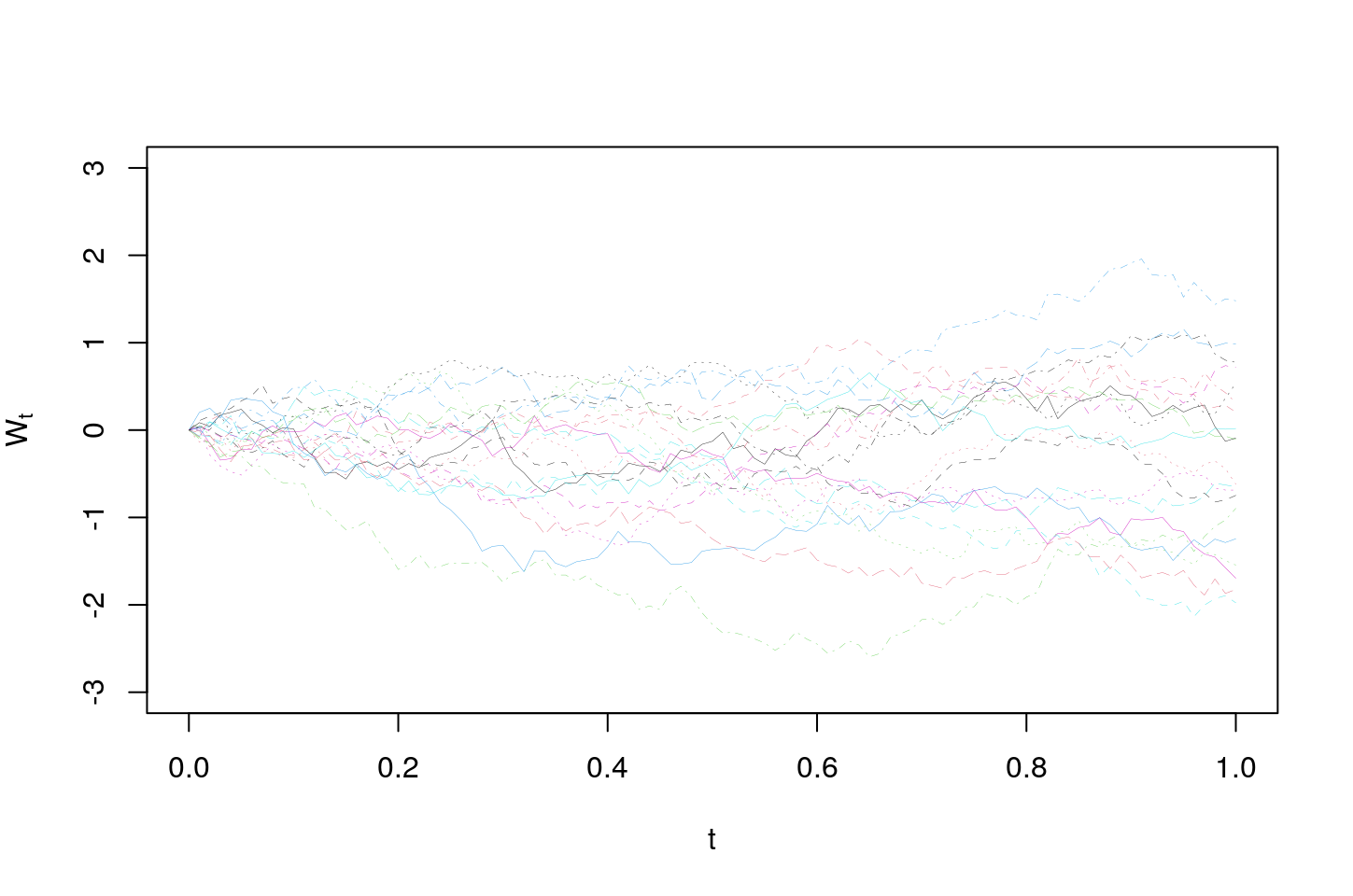
The above algorithm is motivated by the following. Let \(X_i\) be iid from some distribution with zero mean and unit variance. Then the ordinary CLT tells us that \[ \frac{1}{\sqrt{n}} \sum_{i=1}^n X_i \buildrel {\rm d} \over \longrightarrow N(0,1).\] Let us define for each \(n\geq 1\) a stochastic process \(W^n_t\), for \(t\in[0,1]\) by \[ W^n_{t}:= \frac{1}{\sqrt{n}} \sum_{i=1}^{\lfloor nt\rfloor} X_i \] Note that, \(W^n_0\equiv 0\) and by the ordinary CLT \(W_{s+t}^n - W_{t}^n \buildrel {\rm d} \over \longrightarrow N(0,1)\) and the process asymptotically has independent stationary increments as well. The famous Donsker’s functional central limit theorem states that \(W^n_\cdot\) as a function converges to the Brownian motion - but that involves working with a suitable space of functions which makes it definitely doctoral material.
11.2 Brownian Bridge
The Brownian bridge on \([0,1]\) is a stochastic process that can be constructed from a Brownian motion in two ways. Let \(W_t\) for \(t\in[0,1]\) be a Brownian motion. The first manner is to define
\[ B_t=W_t-tW_1, \quad t\in[0,1]. \] Notice that by writing
\[B_t=(1-t)W_t - t(W_1-W_t),\]
and invoking the independent increments property of the Brownian motion we have that \(B_t\) follows a normal distribution with zero mean and variance
\[ (1-t)^2t+t^2(1-t)=t-t^2=t(1-t). \] Using this or otherwise we see that \(B_t\equiv 0\) for \(t\in\{0,1\}\). This is the reason it is called a Brownian Bridge as its paths traveling from zero to zero over \([0,1]\) make them look like bridges. Also,
\[ B_{s+t}-B_{t}=W_{s+t}-W_t -sW_1= -s(W_1-W_{s+t})+(1-s)(W_{s+t}-W_t)-sW_t, \]
with the latter expression, and indepenent, stationary increments of the Brownian motion implying that \(B_{s+t}-B_t\) has a zero mean normal distribution with variance
\[ s^2(1-(s+t))+(1-s)^2s+s^2t=s(1-s) \] But clearly the increments are not independent as the process equals zero at \(0\) and \(1\); algebraically
\[ B_{1/2}-B_0=W_{1/2}-(1/2)W_1=-(B_1-B_{1/2}), \] implying in particular that
\[ {\rm Cov}\left(B_{1/2}-B_0,B_1-B_{1/2}\right)=-1. \] It is a good exercise to show that the Brownian bridge can be alternately defined/constructed as follows:
\[ B_t:=(1-t)W\left(\frac{t}{1-t}\right),\quad t\in[0,1]. \] Note that the above definition requires the paths of the Brownian motion over \([0,\infty)\), unlike the earlier one which required it over the unit interval \([0,1]\). Also, this last definition is interesting as it can be seen as a scaled time change of the Brownian motion.
It is also an easy exercise to show that
\[ {\rm Cov}\left(B_s,B_t\right)=\min(s,t)-st, \quad s,t\geq 0. \]
Finally, we observe that the Brownian bridge can be seen as the Brownian motion over \([0,1]\) conditioned on the event that \(B_1=0\) - this obviously implies the bridge property. This is so as \((W_t,W_1)\) follows a bivariate normal given by, \[ N_2\left(\left(\begin{matrix} 0 \\ 0\end{matrix}\right), \left(\begin{matrix} t & t \\ t & 1 \end{matrix}\right)\right), \] and from the conditional distribution of a coordinate given the other under a bivariate normal, we have \[ W_t|W_1\sim N(tW_1,t(1-t)) \implies W_t-tW_1|W_1\sim N(0,t(1-t)) \implies W_t|W_1=0 \buildrel \rm d \over =W_t-tW_1. \]
We end this section with a plot of \(20\) paths from a Brownian bridge.
N<-100
n<-20
x<-t(apply(matrix(rnorm(n*N,0,1/sqrt(N)),nrow=n),1,cumsum))
x<-cbind(rep(0,n),x)
w<-diag(x[,(N+1)])%*%matrix((0:N)/N,nrow=n,ncol=N+1,byrow=TRUE)
w<-x-w
matplot((0:(N))/N,t(w),ylim=c(-3,3),type="l",lwd=0.2,xlab=TeX('$t$'),ylab=TeX('$B_t'))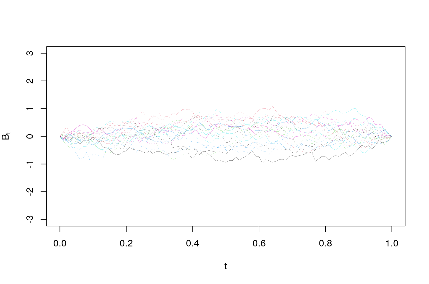
11.3 Convergence of \({\large\sqrt{n}(F_n(\cdot)-F(\cdot))}\)
One of the celebrated results in probability theory is the following Donsker’s invariance principle:
Consider a random sample of size \(n\) from \(U(0,1)\), and let \(F_n(\cdot)\) denote the empirical cdf and let \(F(\cdot)\) denote the cdf of \(U(0,1)\). Then we have, \[ \sqrt{n}(F_n(\cdot)-F(\cdot))\buildrel {\rm d} \over \longrightarrow B_\cdot \]
In the case that the sampling distribution is not \(U(0,1)\) but still a continuous distribution, then the following similar version holds:
\[ \sqrt{n}(F_n(\cdot)-F(\cdot))\buildrel {\rm d} \over \longrightarrow B_{F(\cdot)} \]
These results are similarly useful as the CLT in finding asymptotic distributions of sample statistics - think the delta method - albeit things are a lot more complex as these are limit theorem of random functions instead of the simple random variables or vectors. Below we show some of its applications.
11.4 Kolmogorov-Smirnov Test Statistic
The Kolmogorov-Smirnov test statistic is useful to test if a given random sample arises from a given distribution \(F\). The idea is so look at the statistic
\[ D:=\sqrt{n} \sup_{t\in \mathbb{R}} \vert F_n(\cdot)-F(\cdot)\vert \]
and compare it with its asymptotic limit,
\[ \sup_{t\in \mathbb{R}} \vert B_t\vert. \]
In this case, interestingly the exact distribution of the latter is known, and is given by
\[ 8x\sum_{k\geq 1} (-1)^{(k-1)} k^2 \exp\left\{-2k^2x^2\right\}, \quad x\geq 0. \] But in general can be determined approximately via simulation. The following R code does both, and moreover estimates its \(90\),\(95\) and \(99\)-th percentiles. Comparing these with those in the text on page 331, or otherwise, we see that we need more samples to accurately estimate the \(99\)-th percentile. Of course, in this case since the exact distribution is known, one can use it to derive any percentile - given that I have done a few such exercises, you should be able to do it and share your code via piazza.
p<-c(0.9,0.95,0.99);
maxw<-function(N) {
 W<-cumsum(rnorm(N,0,1/sqrt(N)));
 B<-W-W[N]*(1:N)/N;
 max(abs(B))
}
n<-20000;
sort(mw<-sapply(rep(2000,n),maxw))[p*n] # Finding the sample percentiles
## [1] 1.212355 1.348885 1.605105# Exact Density
exden<-function(x) {
8*x*sum((-1)^(0:99)*(1:100)^2*exp(-2*(1:100)^2*x^2)) # Beware of small values of x for which (1:100) will not suffice
}
plot(xx<-(100:2500)/1000,sapply(xx,exden),col=2,type="l",xlab="x",ylab="Density");
lines(density(mw));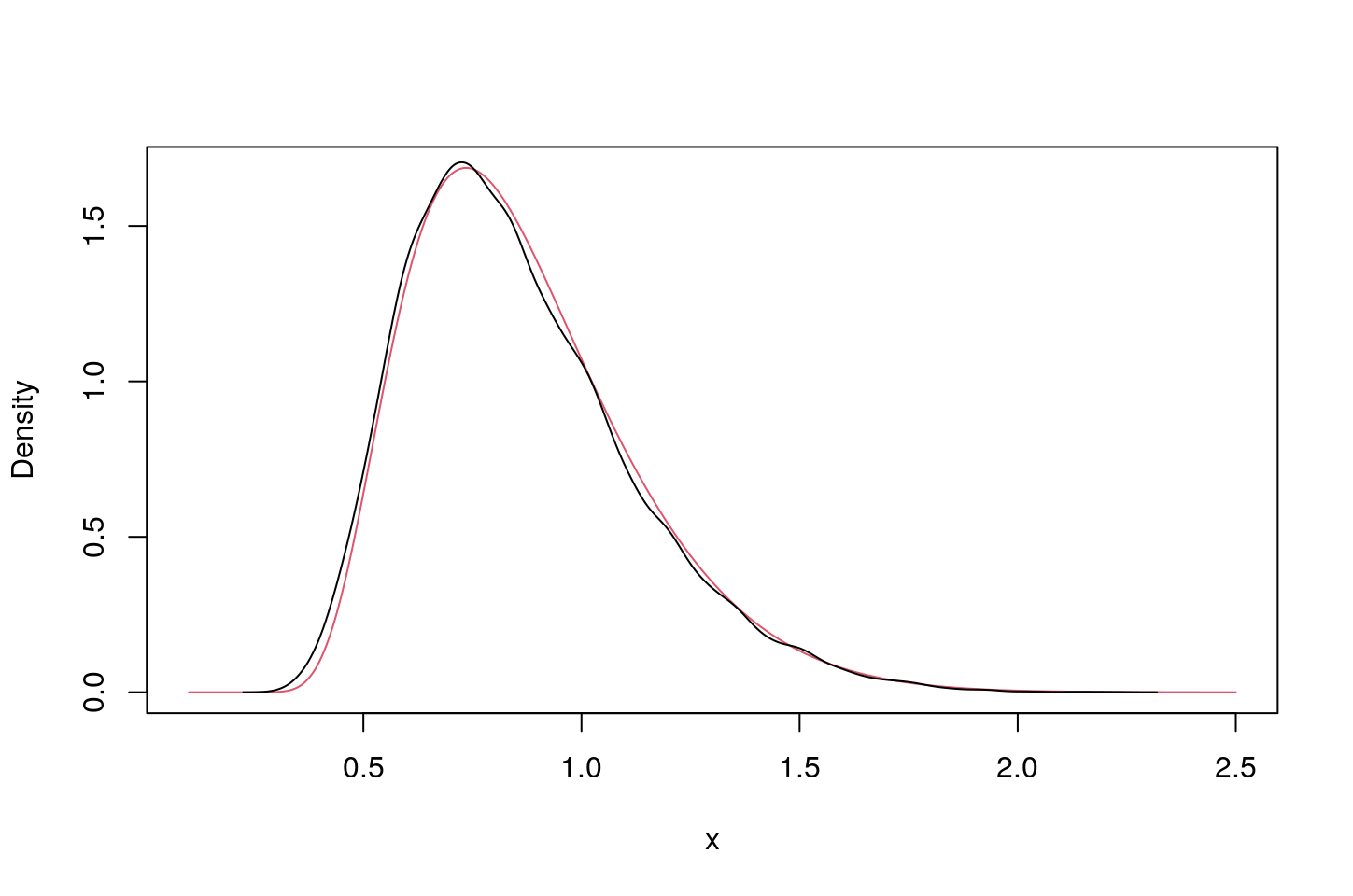
One final comment on how to compute \(D\). Since with probability one the observations are distinct when sampling from a continuous distribution, denoting the order statistics by \(x_{(i)}\), for \(i=1,\ldots,n\) and we note that \(F_n\) is given by
\[ F_n(x)= \frac{i}{n}, \quad x_{(i)}\leq x < x_{(i+1)}; \; i=0,\ldots,n. \]
In the above, we use \(x_{(0)}=-\infty=-x_{(n+1)}\). Hence, \(D\) simplifies to (give it a thought)
\[ D=\max_{1\leq i \leq n} \left(F(x_{(i)})-\frac{i-1}{n}, \frac{i}{n}-F(x_{(i)})\right). \]
11.5 Anderson-Darling Test Statistic
One of the downside of the Kolmogorov-Smirnov statistic is that it does not reflect well the discrepancies near the ends well because of the tendency of the distribution function to approach zero and one at the two ends. To alleviate this issue, the Anderson-Darling test statistic upscales the squared discrepancy \(\sqrt{n}(F_n(x)-F(x))\) by the inverse of \(F(x)(1-F(x))\), with the latter reflecting the variance of \(\sqrt{n}(F_n(x)-F(x))\). The Anderson-Darling statistic is given by
\[ A:=\int_0^\infty \frac{\left(\sqrt{n}(F_n(x)-F(x))\right)^2}{F(x)(1-F(x))}f(x) {\rm d}x. \] Using the convergence to the Brownian bridge, and by change of variables, we see that the above converges to
\[ \int_0^1 \frac{B_t^2}{t(1-t)}{\rm d}t. \]
Using the above observations, we are able to simulate the critical values for the test statistic A below. Compare these values to those in the text on page 333.
p<-c(0.9,0.95,0.99);
ad_func<-function(N) {
 W<-cumsum(rnorm(N,0,1/sqrt(N)));
 B<-W-W[N]*(1:N)/N;
 mean(B[-N]^2*((1:(N-1))/N*(1-(1:(N-1))/N))^{-1})
}
n<-20000;
sort(ad<-sapply(rep(2000,n),ad_func))[p*n] # Finding the sample percentiles
## [1] 1.938458 2.474861 3.890887plot(density(ad),col=1,type="l",xlab="x",ylab="Density",main="");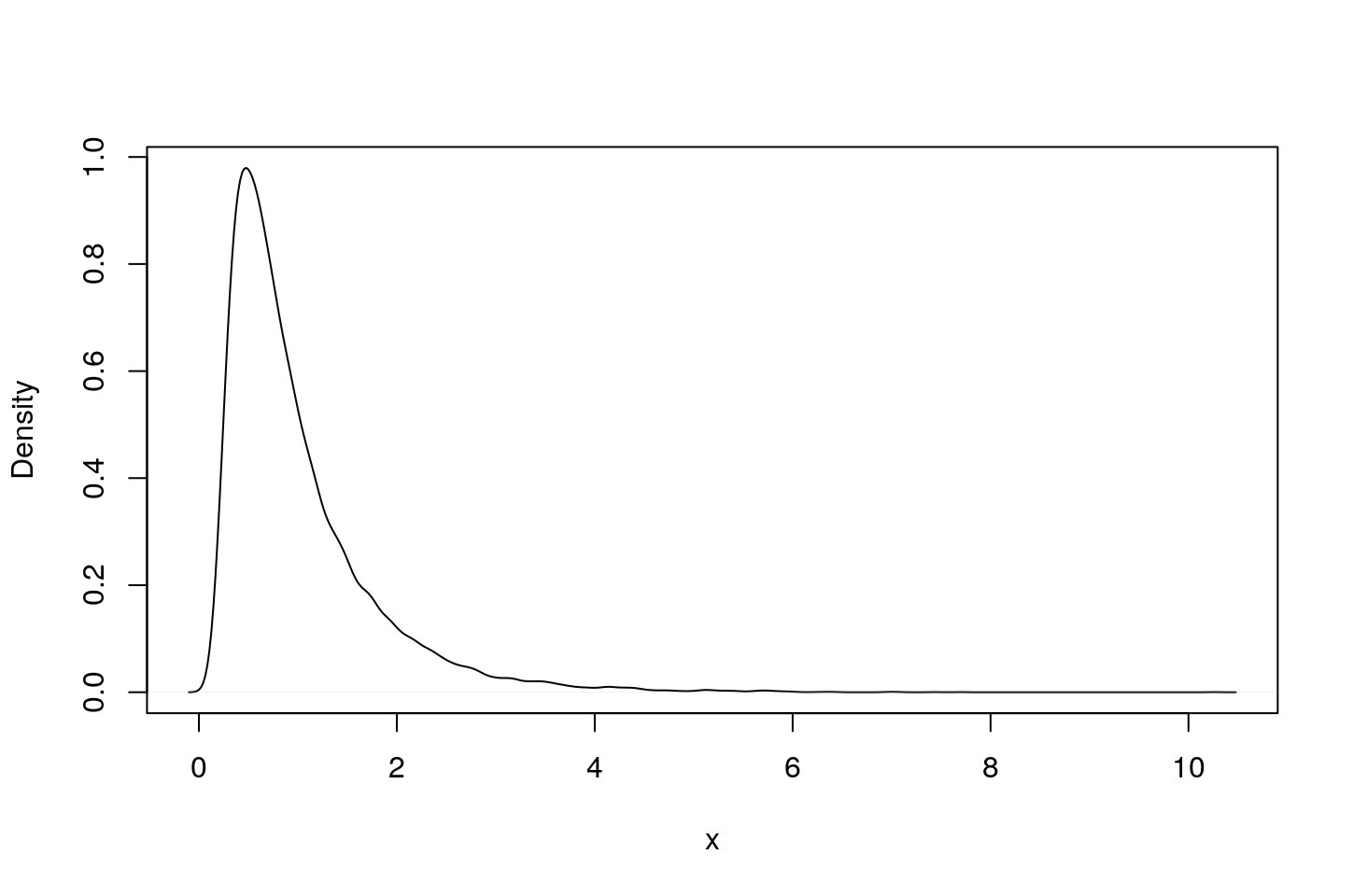
Finally, we derive a simplified representation for the Anderson-Darling statistic, \(A\). For this purpose, we denote the distinct values in the sample by \(y_1<y_2<\ldots<y_k\), and let \(y_0:=0\) and \(y_{k+1}:=u\). Now we have, \[ \begin{aligned} A&=\int_0^u \frac{\left(\sqrt{n}(F_n(x)-F(x))\right)^2}{F(x)(1-F(x))}f(x) {\rm d}x\\ &=n \int_0^u \left([F_n(x)-1]-[F(x)-1]\right)^2\frac{f(x)}{F(x)(1-F(x))} {\rm d}x\\ &=n \int_0^u \left(\left([F_n(x)-1]\right)^2 \left[\frac{f(x)}{F(x)}+\frac{f(x)}{(1-F(x))}\right]+ f(x)\left[\frac{1}{F(x)}-1\right] +2\left(F_n(x)-1\right) \left[\frac{f(x)}{F(x)}\right]\right) {\rm d}x\\ &=n \int_0^u \left(\left([F_n(x)-1]\right)^2 \left[\frac{1}{(1-F(x))}\right] +\left(F_n(x)\right)^2 \left[\frac{1}{F(x)}\right]-1\right) f(x){\rm d}x\\ &=n \sum_{j=0}^k \left([F_n(y_j)-1]\right)^2 \left[\log(1-F(y_j))-\log(1-F(y_{j+1}))\right]\\ &\qquad + n\sum_{j=0}^k \left(F_n(y_j)\right)^2\left[\log F(y_{j+1}) - \log F(y_{j})\right] - nF(u).\\ \end{aligned} \]
11.6 Parting Message
# s<-"Your Message"; #Uncomment this with your message replaced
chr<-function(n) { rawToChar(as.raw(n)) };
asc <- function(x) { strtoi(charToRaw(x),16L) };
#s_asc<-unlist(lapply(unlist(strsplit(s,"")),asc)); uncomment this
s_asc<-c(72,97,118,101,32,97,32,71,114,101,97,116,32,83,117,109,109,101,114,33); # Delete this - I am using this to hide my message!!
s_array<-unlist(lapply(s_asc,chr));
ss<-" ";
for (i in 1:length(s_asc)) {
ss<-paste(ss,s_array[i],sep="");
}
my_s<-unlist(strsplit(ss,""))
par(pty = "s")
plot(c(-1,25), c(-1,25), type = "n", xlab = "", ylab = "", xaxs = "i", yaxs = "i")
title(paste("My Not so Random Message!"));
grid(26, 26, lty = 1);
for(i in 1:(length(s_asc)+1)) {
        x <- floor(runif(1)*25)
        y <- floor(runif(1)*25)
        points(x+0.5, y+0.5, pch = my_s[i],col=floor(runif(1)*10)+1)
}
#print(ss) # Uncomment if you give up!!I had fun teaching and am glad that I ploughed through and developed a lot of e-teaching material … hope you did enjoy listening to a few of the days and working through a few of the e-materials as well!! I wish you a very rewarding career and a quick travel to FSA/FCAS!