7 Bayesian HPD Set
In this note we will discuss the problem of constructing a set, called the credibility set, for a real valued parameter which has a posterior probability of (containing the paramter) \((1-\alpha)\), for a given \(\alpha\in(0,1)\). We will restrict ourselves to the continuous case as the discrete case is similar and only easier computation wise.
We observe that as posed above there exist infinitely many solutions for any \(\alpha\in(0,1)\) - if it is not clear as to why this happens, it will become clear as we proceed along. This then allows us to choose an optimal one among them. Clearly, all of them have the same posterior probability; hence we need another criterion to choose the preferred one among them. A natural such criterion in the case of a real valued parameter is to prefer a shorter in length set. In other words, the shortest in length set with posterior probability of \((1-\alpha)\) is our optimal credibility set of level \((1-\alpha)\). The question then is to how to determine this set in practice.
7.1 General Result
We state and prove a general result by abstracting a bit as follows. Note that the posterior density for a real valued parameter is a density on \(\mathbb{R}\). Also, note that the length of an arbitrary set \(C\) can be defined as \[ \int I_C(\theta) {\rm d}\theta, \] where \(I_C(\cdot)\) is the indicator function for the set \(C\), i.e. \(1\) on \(C\) and \(0\) otherwise.
Theorem Let \(f\) denote a density on \(\mathbb{R}\). Then for \(\alpha\in (0,1)\), a set \(C\) with the shortest length among those with \(f\) probability equal to \(1-\alpha\) equals \[ C_\alpha:=\left\{f>c_\alpha \right\} \cup E, \] from some \(c_\alpha>0\) and \(E\subseteq \left\{f=c_\alpha \right\}\). \(\blacksquare\)
We note that in applications, the set \(\left\{f=c \right\}\), for any \(c>0\), would contain atmost a finite many elements; in such cases, the set \(E\) can be taken to be the empty set, i.e. \[ C_\alpha:=\left\{f>c_\alpha \right\}, \] from some \(c_\alpha>0\). An extreme case where \(E\) is not empty for any \(\alpha\in(0,1)\) is when \(f\) is a uniform density - but a uniform density does not arise as a posterior density.
Proof of the theorem: We will break the proof into the following two steps. The second step is the more important one from a practical insight perspective; the first is for those motivated to strive towards a full understanding.
The existence of \(c_\alpha\): Consider the set \(D_c\) defined for \(c\geq 0\) as
\[
D_c:=\left\{f>c \right\}.
\]
We note that \({\rm Pr}\left(D_c\right)\) under \(f\) is a right continuous function of \(c\) as it is the survival function of the density (as the random variable). The points of discontinuity are the level sets of \(f\) which have a positive probability under \(f\), i.e. values of \(c\) such that
\[
\int I_{\left\{\eta:f(\eta)=c\right\}}(\theta) f(\theta) {\rm d}\theta >0.
\]
To see this let we note that since \(\psi\) defined by \(\psi(c):={\rm Pr}\left(D_c\right)\) is a decreasing function of \(c\) with \(\psi(0)=1\) \(\lim_{c\rightarrow\infty}\psi(c)=0\), there either exists a \(c_\alpha\) such that \(C_\alpha:=\left\{f>c_\alpha \right\}\) satisfies
\[
\int I_{C_\alpha}(\theta) f(\theta) {\rm d}\theta =1-\alpha,
\]
or
\[
\psi(c_\alpha-)\geq(1-\alpha)>\psi(c_\alpha).
\]
In the latter case, using a technical result from measure theory (that the Lebesgue measure is nonatomic; I teach this in my Fall PhD level course on probability theory), it can be shown that a subset \(E\) of \(\{\eta:f(\eta)=c_\alpha\}\) can be carved such that
\[
C_\alpha:=\left\{f>c_\alpha \right\} \cup E,
\]
has \(f\) probability \(1-\alpha\).
The Optimality of \(C_\alpha\): Observe that since \(c_\alpha>0\), \[ \int I_{C_\alpha}(\theta) {\rm d}\theta\leq \int I_{C_\alpha}(\theta) \frac{f(\theta)}{c_\alpha}{\rm d}\theta\leq \frac{1-\alpha}{c_\alpha}<\infty. \] We begin by showing that for any set \(C\) with the same length as \(C_\alpha\) has \(f\) probability atmost \((1-\alpha)\), i.e. \({\rm Pr}\left(C_\alpha\right)\geq {\rm Pr}\left(C\right)\). Note that this is equivalent to showing that \({\rm Pr}\left(C_\alpha\cap {C}^{\mathsf{c}}\right)\geq {\rm Pr}\left(C\cap {C_\alpha}^{\mathsf{c}}\right)\). This is true since the lengths of \(C_\alpha\cap {C}^{\mathsf{c}}\) equals that of \(C\cap {C_\alpha}^{\mathsf{c}}\) and moreover, \[ C_\alpha\cap {C}^{\mathsf{c}}\subseteq \{\eta:f(\eta)\geq c_\alpha\} \quad \hbox{and} \quad C\cap {C_\alpha}^{\mathsf{c}}\subseteq \{\eta:f(\eta)\leq c_\alpha\}. \] More clearly, \[ \begin{aligned} {\rm Pr}\left(C_\alpha\cap {C}^{\mathsf{c}}\right)&=\int_{C_\alpha\cap {C}^{\mathsf{c}}} f(\theta){\rm d}\theta\\ &\geq c_\alpha \int_{C_\alpha\cap {C}^{\mathsf{c}}} {\rm d}\theta\\ &= c_\alpha \int_{C\cap {C_\alpha}^{\mathsf{c}}} {\rm d}\theta\\ &\geq \int_{C\cap {C_\alpha}^{\mathsf{c}}} f(\theta){\rm d}\theta={\rm Pr}\left(C\cap {C_\alpha}^{\mathsf{c}}\right).\\ \end{aligned} \] This implies that any other candidate \((1-\alpha)\) level credible set \(C\) has atleast the same length as \(C_\alpha\). This is so as other wise \(C\) can be augmented to increase its length to that of \(C_\alpha\) (using if need be non-atomicity of the Lebesgue measure), which will result in a post-augmentation probability under \(f\) of \(C\) being strictly greter than \((1-\alpha)\) - a contradiction to the above. \(\blacksquare\)
Note: It can be shown that any shortest length set \(C\) is essentially of the above form with a bit more effort, but since that is not practically relevant we will leave it for the motivated reader to either prove it themselves or discuss it during office hours.
7.2 Highest Posterior Density (HPD) Credible Set
Note that the above general result implies that the above \(C_\alpha\) is a shortest length \((1-\alpha)\) level credible set for a parameter \(\theta\), constructed with the posterior density of \(\theta\), denoted by \(\pi(\cdot|\tilde{x})\), replacing \(f\) above.
Now we turn to defining the above \(C_\alpha\) in practice via computing the \(c_\alpha\) - the cases we will look at will be such that the level sets of the posterior would be sets with finitely many elements, so the \(E\) above could be taken to be the empty set.
Note that mathematically the HPD set is easily defined if the posterior density is non-increasing from the left-end point of its support - in this case it will be an interval from this left-end point of its support to its \((1-\alpha)\)-th quantile. In the example above this observation can be used to construct the HPD set. But because of the Bayesian CLT (see Theorem 15.16 of the text), which is called the Bernstein von-Mises theorem, we see that but for these pathological cases the posterior will approach normal and hence its density is unlikely to be non-increasing. So this mathematically interesting case is not statistically or practically of much use.
On the other hand, asymptotic normality suggests that a good class of posteriors to look at will be those which are unimodal. But before we do this, we comment that if the posterior is a symmetric unimodal then the HPD will be constructed by solving for \(y\) such that
\[
(1-\alpha)=F(\hbox{posterior mode}+y)-F(\hbox{posterior mode}-y)=2*F(mode+y)-1,
\]
where \(F\) denotes the posterior. Note that suc a \(y\) is given by
\[
y=F^{-1}(1-\alpha/2)-\hbox{posterior mode},
\]
which can be computed if \(F^{-1}\) is available (like qnorm) or by using a root finding function like uniroot.
7.2.1 Unimodal Posterior Density
Let us consider the case of a random sample \(X_i\), \(i=1,\ldots,n\), from \(Bin(m,p)\). The conjugate prior for this model is the beta distribution, and let us suppose that our beta prior has parameters \(\alpha\) and \(\beta\) and mean \(\alpha/(\alpha+\beta)\). Then it is easy to check that the posterior distribution is also a beta with parameters \(\alpha+\sum x_i\) and \(\beta+mn-\sum x_i\). In the following we fix the likelihood to be that of \(Bin(2,2/3)\), and the prior to be \(Beta(3,3)\).
7.2.1.1 Dynamic Simulation
We begin first by a simulation to show that the posterior \(p\) increasingly concentrates at \(2/3\) with rising sample size. Also, note that by the Bernstein von-Mises Bayesian CLT, the posterior of \(p\) centered at the MLE \(\hat{p}\) and scaled by \(\sqrt{n}\), with \(\hat{p}\) given by
\[
\hat{p}=\bar{X}/2
\]
increasingly approaches the normal distribution with zero mean and variance given by the asymptotic variance of the MLE, which in this case equals \(1/3\). The below dynamic simulation using shiny demonstrates this quite visibly - click the play button!
If you are interested in creating such apps, look at this tutorial. The code that I use is as follows, and was motivated by an effort by one of our doctoral students in Actuarial Science, Abylay Zhexembay:
User Interface Code:
```
shinyUI(fluidPage(
    titlePanel("Posterior distribution"),
    sidebarLayout(
        sidebarPanel(
            sliderInput(inputId = "size", label = "Sample size:", min = 0,
                        max = 1000, value = 0,
                        animate = animationOptions(100))),
        mainPanel(plotOutput(outputId = "Plot1",width="100%"),
                  plotOutput(outputId = "Plot2",width="100%"))
        )))
Server Side Code:
```
library(shiny);
library(latex2exp);

shinyServer(function(input, output, session) {
    session$onSessionEnded(function() shiny::stopApp())
    p <- 2/3
    x <- rbinom(1000,2, p)
    y <- seq(0, 1, 0.01)
    output$Plot1 <- renderPlot({
        plot(y, dbeta(y, 3+sum(x[0 : input$size]),3+2*input$size-sum(x[0 : input$size])),
             type = "l", ylab=TeX("$\\pi(p|\\tilde{x})$"), xlab="p",ylim = c(0, 50),main="Actual Beta Posterior")},height=400,width=400)

    output$Plot2 <- renderPlot({
        plot(y<-seq(-2, 2, 0.01), dbeta(y/sqrt(input$size)+mean(x[0 : input$size])/2, 3+sum(x[0 : input$size]),3+2*input$size-sum(x[0 : input$size]))/sqrt(input$size),
             type = "l", ylab=TeX("Density"), xlab=TeX("Posterior of $\\sqrt{n}(p-\\hat{p})$"), ylim = c(0, 2),
             main=TeX("Posterior Centered at MLE and scaled by $\\sqrt{n}$"))
        lines(y<-seq(-2, 2, 0.01),dnorm(y,mean=0,sd=1/(3)),col=4)
    legend("topleft", legend=c("N(0,1/3)", TeX("Posterior of $\\sqrt{n}(p-\\hat{p})$")),
           col=c("blue", "black"),lty=rep(1,2))},height=400,width=400)
})
7.2.1.2 Computing the HPD
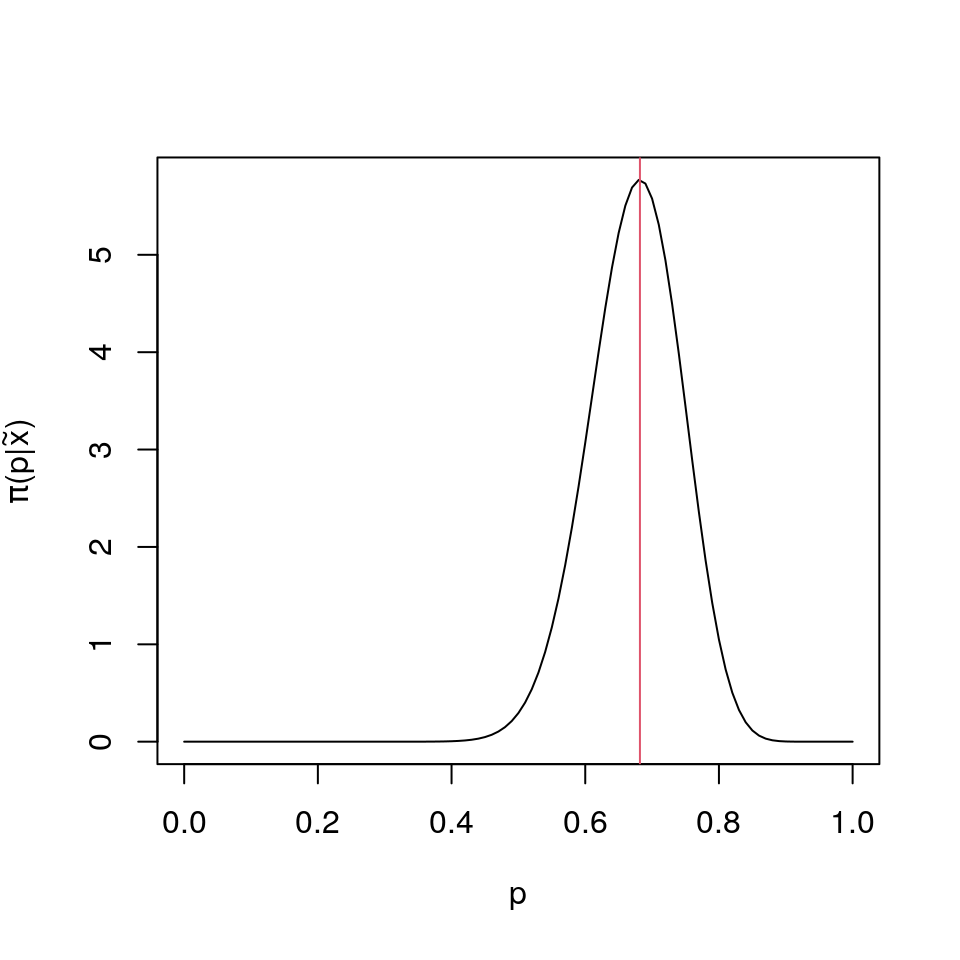
To fix things we simulate a \(20\) sample from the above chosen \(Bin(2,2/3)\), and plot its posterior for the mentioned \(Beta(3,3)\) prior. Note that the posterior is a beta distribution again, as beta is a conjugate prior for the binomial model, and is given by \[ Beta\left(3+\sum_{i=1}^n x_i, 3+2*20-\sum_{i=1}^n x_i\right) \]
set.seed("19846")
x<-rbinom(20,2,2/3);
and notice that the posterior beta parameters are 31 and 15, and hence with mode 0.682.
library(latex2exp)
plot(p<-(0:100)/100,dbeta(p,3+sum(x),3+2*20-sum(x)),type="l",xlab=TeX("$p$"),ylab=TeX("$\\pi(p|\\tilde{x})$"));
lines(rep((2+sum(x))/44,2),c(-1,7),col=2)library(rootSolve)
# Value of the Posterior Density at its Mode
ul<-dbeta(pmode<-(2+sum(x))/44,alpha<-3+sum(x),beta<-43-sum(x));
# Workhorse Function
prob_candidate<-function(c){
dum<-function(z){
dbeta(z,alpha,beta)-c
}
limits<-uniroot.all(dum,c(0,1))
pbeta(limits[2],alpha,beta)-pbeta(limits[1],alpha,beta)-0.95
}
# Computing the HPD
c95<-uniroot(prob_candidate,c(0.0001,ul-0.1))$root
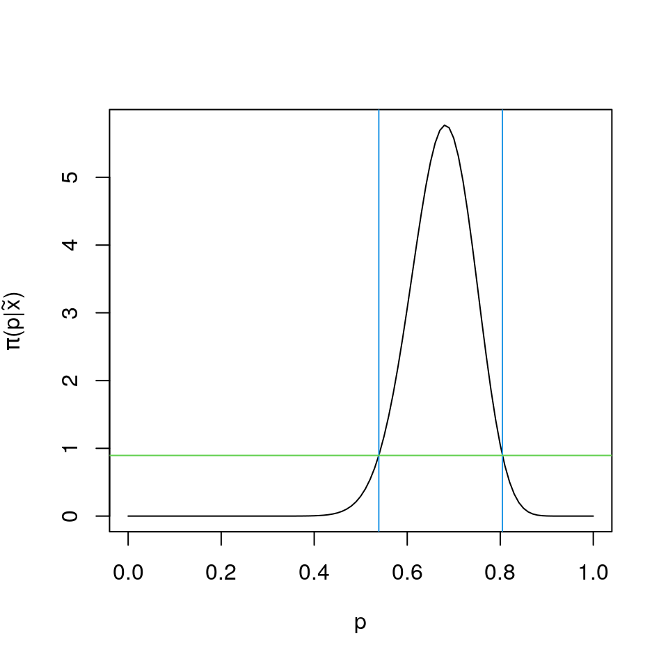
hpd<-uniroot.all(function(z){dbeta(z,alpha,beta)-c95},c(0,1))The computed 95% HPD interval has its lower and upper limits as 0.5389, 0.8046, and its exact coverage probability is 0.9500005.
library(latex2exp)
plot(p<-(0:100)/100,dbeta(p,3+sum(x),3+2*20-sum(x)),type="l",xlab=TeX("$p$"),ylab=TeX("$\\pi(p|\\tilde{x})$"));
lines(rep(hpd[1],2),c(-1,7),col=4)
lines(rep(hpd[2],2),c(-1,7),col=4)
lines(c(-1,2),rep(dbeta(hpd[1],alpha<-3+sum(x),beta<-43-sum(x)),2),col=3)
We end this note by observing that in general the HPD credible set need not be an interval when the posterior is not unimodal - unimodality implies it will be an interval though (prove it!).