Chapter 10 Markov Chain Monte Carlo

10.1 Simulation with Dependent Observations

Suppose we want to compute

\[\begin{equation*} \theta = E[h(X)] = \int h(x) f(x) dx \end{equation*}\]

Crude Monte Carlo: generate \(X_1,\dots,X_N\) that are

• independent;
• identically distributed from \(f\).

and compute \(\widehat{\theta} = \frac{1}{N} \sum h(X_i)\).

Then

• \(\widehat{\theta} \to \theta\) by the law of large numbers;
• \(\widehat{\theta} \sim \text{AN}(\theta, \sigma^2/N)\) by the central limit theorem;
• \(\sigma^2\) can be estimated using the sample standard deviation.

Sometimes generating independently from \(f\) is not possible or too costly.

Importance sampling: generate independently from \(g\) and reweight.

Alternative: generate dependent samples in a way that

• preserves the law of large numbers;
• has a central limit theorem if possible.

Variance estimation will be more complicated.

10.2 A Simple Example

Suppose \(X,Y\) are bivariate normal with mean zero, variance 1, and correlation \(\rho\),

\[\begin{equation*} (X,Y) \sim \text{BVN}(0,1,0,1,\rho). \end{equation*}\]

Then

\[\begin{align*} Y|X=x &\sim \text{N}(\rho x, 1-\rho^2)\\ X|Y=y &\sim \text{N}(\rho y, 1-\rho^2). \end{align*}\]

Suppose we start with some initial values \(X_0, Y_0\) and generate

\[\begin{align*} X_1 &\sim \text{N}(\rho Y_0, 1-\rho^2)\\ Y_1 &\sim \text{N}(\rho X_1, 1-\rho^2) \end{align*}\]

(\(X_0\) is not used), and continue for \(i = 1, \dots, N-1\)

\[\begin{align*} X_{i+1} &\sim \text{N}(\rho Y_i, 1-\rho^2)\\ Y_{i+1} &\sim \text{N}(\rho X_{i+1}, 1-\rho^2)\\ \end{align*}\]

For \(\rho = 0.75\) and \(Y_0 = 0\):

r <- 0.75
x <- numeric(10000)
y <- numeric(10000)
x[1] <- rnorm(1, 0, sqrt(1 - r^2))
y[1] <- rnorm(1, r * x[1], sqrt(1 - r^2))
for (i in 1:(length(x) - 1)) {
    x[i+1] <- rnorm(1, r * y[i], sqrt(1 - r^2))
    y[i+1] <- rnorm(1, r * x[i + 1], sqrt(1 - r^2))
}

The joint distribution of \(X\) and \(Y\) and the marginal distribution of \(X\) look right; the marginal distribution of \(Y\) does as well.

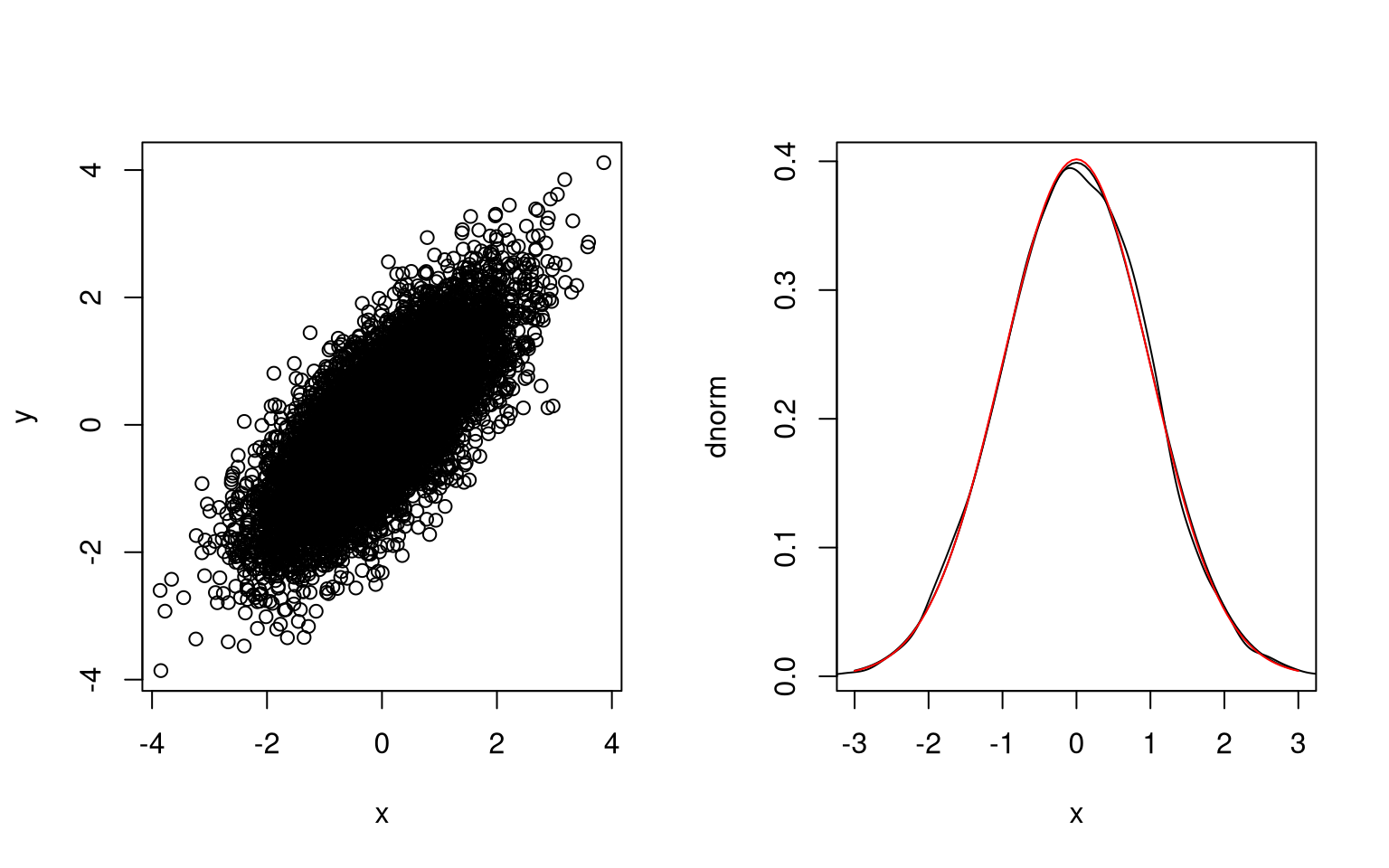
The correlation is close to the target value:

cor(x,y)
## [1] 0.743805

Initial sample paths show the dependence:

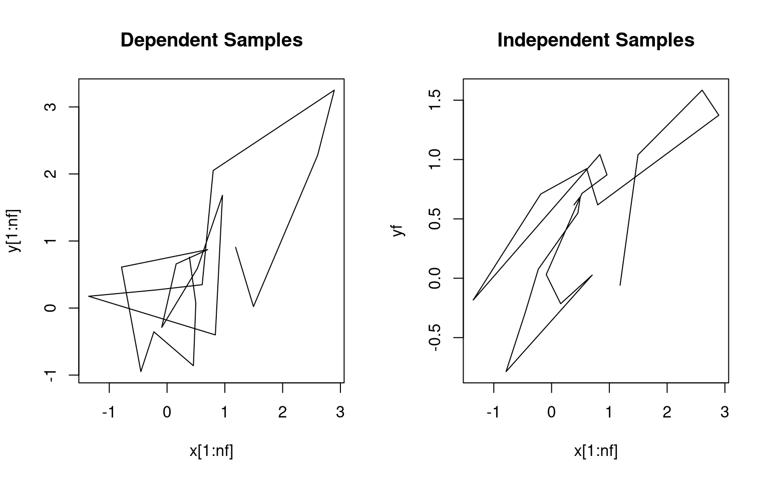
The sample auto-correlation function for \(X\) also reflects the dependence:

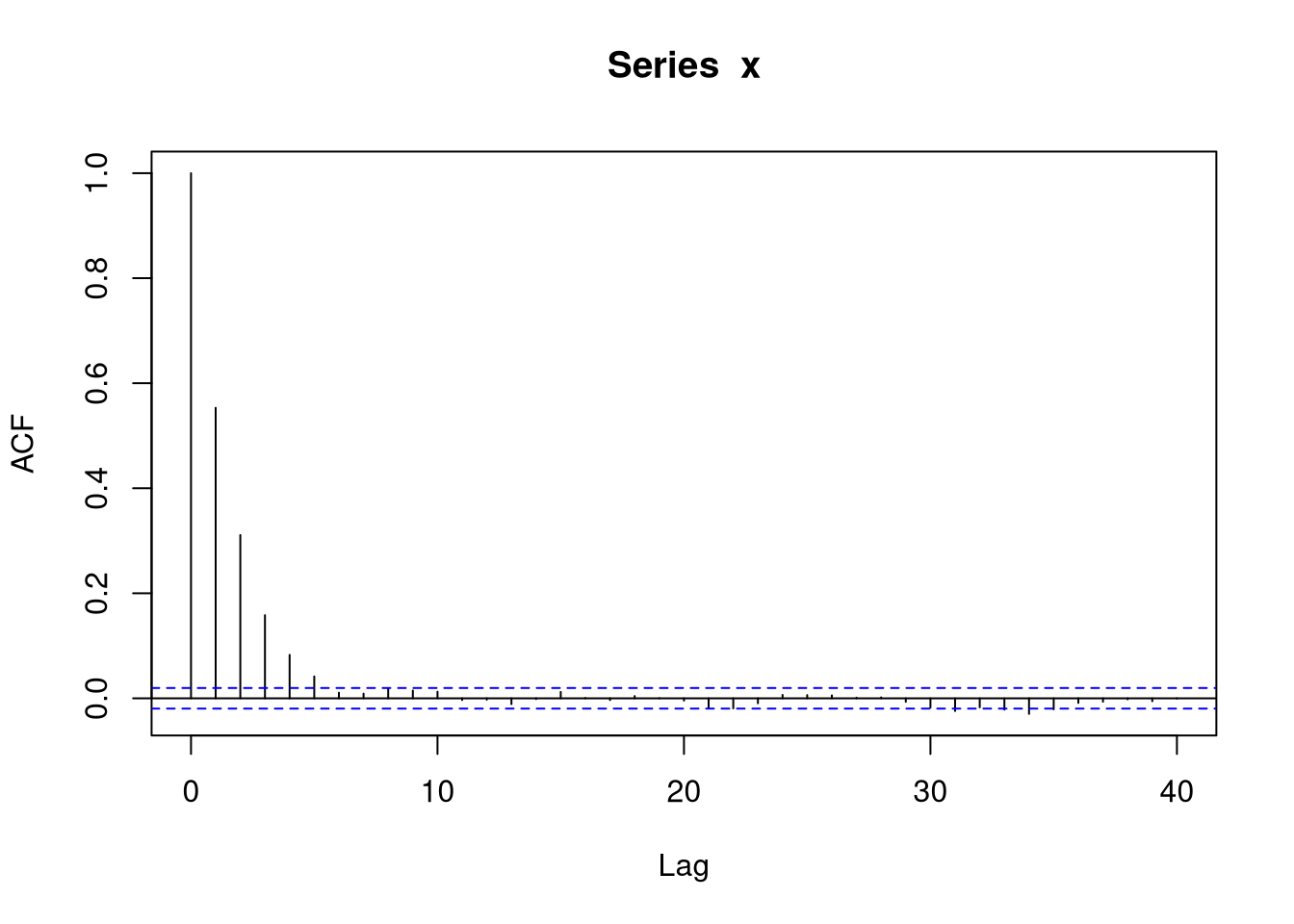
The sequence of pairs \((X_i,Y_i)\) form a continuous state space Markov chain.

Suppose \((X_0,Y_0) \sim \text{BVN}(0,1,0,1,\rho)\). Then

• \((X_1,Y_0) \sim \text{BVN}(0,1,0,1,\rho)\);
• \((X_1,Y_1) \sim \text{BVN}(0,1,0,1,\rho)\);
• \((X_2,Y_1) \sim \text{BVN}(0,1,0,1,\rho)\);
• \(\dots\)

So \(\text{BVN}(0,1,0,1,\rho)\) is a stationary distribution or invariant distribution of the Markov chain.

\(\text{BVN}(0,1,0,1,\rho)\) is also the equilibrium distribution of the chain, i.e. for any starting distribution the joint distribution of \((X_n,Y_n)\) converges to the \(\text{BVN}(0,1,0,1,\rho)\) distribution.

For this example, \(X_1, X_2, \dots\) is an AR(1) process

\[\begin{equation*} X_i = \rho^2 X_{i-1} + \epsilon_i \end{equation*}\]

with the \(\epsilon_i\) independent and \(N(0, 1-\rho^4)\).

Standard time series results show that the equilibrium distribution of this chain is \(\text{N}(0,1)\).

If

\[\begin{equation*} \overline{X}_N = \frac{1}{N}\sum_{i=1}^N X_i \end{equation*}\]

then

\[ \text{Var}({\overline{X}_N}) \approx \frac{1}{N} \frac{1-\rho^4}{(1-\rho^2)^2} = \frac{1}{N}\frac{1+\rho^2}{1-\rho^2} \]

10.3 Markov Chain Monte Carlo

The objective is to compute

\[\begin{equation*} \theta = E[h(X)] = \int h(x) f(x) dx \end{equation*}\]

Basic idea:

• Construct a Markov chain with invariant distribution \(f\).
• Make sure the chain has \(f\) as its equilibrium distribution.
• Pick a starting value \(X_0\).
• Generate \(X_1, \dots, X_N\) and compute \[\begin{equation*} \widehat{\theta} = \frac{1}{N} \sum h(X_i) \end{equation*}\]
• Possibly repeat independently several times, maybe with different starting values.

Some issues:

• How to construct a Markov chain with a particular invariant distribution.
• How to estimate the variance of \(\widehat{\theta}\).
• What value of \(N\) to use.
• Should an initial portion be discarded; if so, how much?

10.4 Some MCMC Examples

Markov chain Monte Carlo (MCMC) is used for a wide range of problems and applications:

• generating spatial processes;
• sampling from equilibrium distributions in physical chemistry;
• computing likelihoods in missing data problems;
• computing posterior distributions in Bayesian inference;
• optimization, e.g. simulated annealing;
• \(\dots\)

10.4.1 Strauss Process

The Strauss process is a model for random point patterns with some regularity.

A set of \(n\) points is distributed on a region \(D\) with finite area or volume.

The process has two parameters, \(c \in [0,1]\) and \(r > 0\). The joint density of the points is

\[\begin{equation*} f(x_1,\dots,x_n) \propto c^\text{number of pairs within $r$ of each other} \end{equation*}\]

For \(c = 0\) the density is zero if any two points are withing \(r\) of each other.

Simulating independent draws from \(f\) is possible in principle but very inefficient.

A Markov chain algorithm:

• Start with \(n\) points \(X_1, \dots, X_n\) with \(f(X_1,\dots,X_n) > 0\).
• Choose an index i at random, remove point \(X_i\), and replace it with a draw from \[\begin{equation*} f(x|x_1,\dots,x_{i-1},x_{i+1},\dots,x_n) \propto c^\text{number of remaining $n-1$ points within $r$ of $x$} \end{equation*}\]
• This can be sampled reasonably efficiently by rejection sampling.
• Repeat for a reasonable number of steps.

Strauss in package spatial implements this algorithm. [Caution: it used to be easy to hang R because the C code would go into an infinite loop for some parameters. More recent versions may have modified C code that checks for interrupts.]

The algorithm is due to Ripley (1979); Ripley’s algorithm applies to a general multivariate density.

10.4.2 Markov Random Fields

A Markov random field is a spatial process in which

• each index \(i\) has a set of neighbor indices \(N_i\);
• \(X_i\) and \(\{X_k: \text{$k \neq i$ and $k \not \in N_i$}\}\) are conditionally independent given \(\{X_j: j \in N_i\}\).

In a binary random field the values of \(X_i\) are binary.

Random fields are used as models in

• spatial statistics;
• image processing;
• \(\dots\)

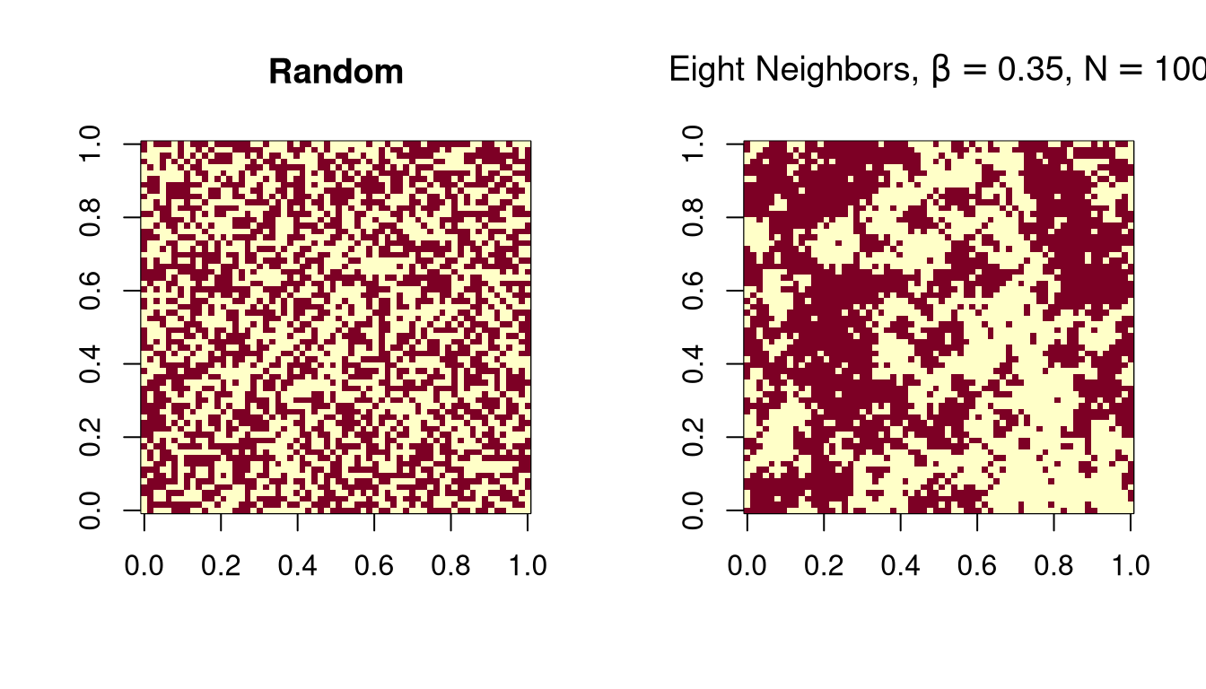
A simple model for an \(n \times n\) image with \(c\) colors:

\[\begin{equation*} f(x) \propto \exp\{\beta\times (\text{number of adjacent pixel pairs with the same color})\} \end{equation*}\]

This is called a Potts model.

For a pixel \(i\), the conditional PMF of the pixel color \(X_i\) given the other pixel colors, is

\[\begin{equation*} f(x_i|\text{rest}) \propto \exp\{\beta \times ( \text{number of neighbors with color $x_i$}\} \end{equation*}\]

10.4.3 Simple Image Reconstruction

Suppose a binary image is contaminated with noise.

The noise process is assumed to act independently on the pixels.

Each pixel is left unchanged with probability \(p\) and flipped to the opposite color with probability \(1-p\).

The likelihood for the observed image \(Y_i\) is

\[\begin{equation*} f(y|x) \propto p^m (1-p)^{n^2-m} \end{equation*}\]

with \(m\) the number of pixels with \(y_i = x_i\).

A Markov random field is used as the prior distribution of the true image.

The posterior distribution of the true image is

\[\begin{equation*} f(x|y) \propto p^m (1-p)^{n^2-m} e^{\beta w} \end{equation*}\]

with \(w\) the number of adjacent pixel pairs in the true image \(x\) with the same color.

The posterior distribution is also a Markov random field, and

\[\begin{equation*} f(x_i|y, \text{$x_j$ for $j \neq i$}) \propto p^{m_i}(1-p)^{1-m_i} e^{\beta w_i} \end{equation*}\]

with \(m_i = 1\) if \(x_i = y_i\) and \(m_i = 0\) otherwise, and \(w_i\) the number of neighbors with color \(x_i\).

Images drawn from the posterior distribution can be averaged to form a posterior mean.

The posterior mean can be rounded to a binary image.

Many other variations are possible.

Another example using \(\beta = 0.5\) and \(\beta = 0.35\) and \(N=100\) will be shown in class.

This is a simple version of the ideas in

Geman, S. and Geman D, (1984) Stochastic relaxation, Gibbs distributions and the Bayesian restoration of images, IEEE Transactions on Pattern Analysis and Machine Intelligence 6, 721–741.

The posterior distributions are related to Gibbs distributions in physics.

Geman and Geman call the Markov chain algorithm Gibbs sampling.

10.4.4 Code for the Image Sampler

simImg <- function (m, img, N, beta, p) {
    colors <- 1:2
    inboff <- c(-1, -1, -1,  0, 0,  1, 1, 1)
    jnboff <- c(-1,  0,  1, -1, 1, -1, 0, 1)
    for (k in 1:N) {
        for (i in 1:nrow(m)) {
            for (j in 1:ncol(m)) {
                w <- double(length(colors))
                inb <- i + inboff
                jnb <- j + jnboff
                omit <- inb == 0 | inb == nrow(m) + 1 |
                        jnb == 0 | jnb == ncol(m) + 1
                inb <- inb[!omit]
                jnb <- jnb[!omit]
                for (ii in 1:length(inb)) {
                    kk <- m[inb[ii], jnb[ii]]
                    w[kk] <- w[kk] + 1
                }
                if (is.null(img)) lik <- 1
                else lik <- ifelse(img[i,j]==colors, p, 1-p)
                prob <- lik * exp(beta * w)
                m[i, j] <- sample(colors, 1, TRUE, prob = prob)
            }
        }
    }
    m
}

10.4.5 Profiling to Improve Performance

Rprof can be used to turn on profiling.

During profiling a stack trace is written to a file, Rprof.out by default, 50 times per second.

summaryRprof produces a summary of the results.

Rprof();system.time(simImg(m,img,100,.35,.7));Rprof(NULL)
##    user  system elapsed 
##  14.671   0.053  14.799
s <-  summaryRprof()
head(s$by.self)
##                   self.time self.pct total.time total.pct
## "simImg"               7.06    47.07      14.74     98.27
## "ifelse"               2.26    15.07       2.78     18.53
## "sample.int"           1.68    11.20       1.82     12.13
## "standardGeneric"      1.42     9.47       1.70     11.33
## "sample"               0.72     4.80       2.60     17.33
## "which"                0.44     2.93       0.44      2.93

Replacing ifelse in

else lik <- ifelse(img[i,j]==colors, p, 1-p)

with

else if (img[i, j] == 1) lik <- c(p, 1-p)
else lik <- c(1 - p, p)

speeds things up somewhat:

Rprof();system.time(simImg1(m,img,100,.35,.7));Rprof(NULL)
##    user  system elapsed 
##  11.079   0.030  11.165
s1 <- summaryRprof()
head(s1$by.self)
##                   self.time self.pct total.time total.pct
## "simImg1"              6.34    55.71      11.12     97.72
## "sample.int"           1.56    13.71       1.66     14.59
## "standardGeneric"      1.42    12.48       1.74     15.29
## "sample"               0.66     5.80       2.38     20.91
## "double"               0.34     2.99       0.36      3.16
## "gc"                   0.26     2.28       0.26      2.28

Starting profiling with

Rprof(line.profiling = TRUE)

will enable source profiling if our funciton is defined in a file and sourced.

Using the package proftools with

library(proftools)
pd <- readProfileData()
annotateSource(pd)

produces

         :  simImg1 <- 
         :  function (m, img, N, beta, p) 
         :  {
         :      colors <- 1:2
         :      inboff <- c(-1, -1, -1, 0, 0, 1, 1, 1)
         :      jnboff <- c(-1, 0, 1, -1, 1, -1, 0, 1)
         :      for (k in 1:N) {
         :          for (i in 1:nrow(m)) {
  0.36%  :              for (j in 1:ncol(m)) {
  4.49%  :                  w <- double(length(colors))
  0.90%  :                  inb <- i + inboff
  1.26%  :                  jnb <- j + jnboff
 25.49%  :                  omit <- inb == 0 | inb == nrow(m) + 1 | jnb == 
         :                    0 | jnb == ncol(m) + 1
  2.69%  :                  inb <- inb[!omit]
  1.80%  :                  jnb <- jnb[!omit]
  2.15%  :                  for (ii in 1:length(inb)) {
  2.15%  :                    kk <- m[inb[ii], jnb[ii]]
  2.69%  :                    w[kk] <- w[kk] + 1
         :                  }
  3.41%  :                  if (is.null(img)) 
         :                    lik <- 1
         :                  else if (img[i, j] == 1) 
         :                    lik <- c(p, 1 - p)
         :                  else lik <- c(1 - p, p)
  1.80%  :                  prob <- lik * exp(beta * w)
 50.45%  :                  m[i, j] <- sample(colors, 1, TRUE, prob = prob)
         :              }
         :          }
         :      }
         :      m
         :  }

This suggests one more useful change: move the loop-invariant computations nrow(m)+1 and ncol(m)+1 out of the loop:

simImg2 <- function (m, img, N, beta, p) {
    colors <- 1:2
    inboff <- c(-1, -1, -1, 0, 0, 1, 1, 1)
    jnboff <- c(-1, 0, 1, -1, 1, -1, 0, 1)
    nrp1 <- nrow(m) + 1
    ncp1 <- ncol(m) + 1
    for (k in 1:N) {
        for (i in 1:nrow(m)) {
            for (j in 1:ncol(m)) {
                w <- double(length(colors))
                inb <- i + inboff
                jnb <- j + jnboff
                omit <- inb == 0 | inb == nrp1 |
                        jnb == 0 | jnb == ncp1
                inb <- inb[!omit]
                jnb <- jnb[!omit]
                for (ii in 1:length(inb)) {
                  kk <- m[inb[ii], jnb[ii]]
                  w[kk] <- w[kk] + 1
                }
                if (is.null(img)) 
                  lik <- 1
                else if (img[i, j] == 1) 
                  lik <- c(p, 1 - p)
                else lik <- c(1 - p, p)
                prob <- lik * exp(beta * w)
                m[i, j] <- sample(colors, 1, TRUE, prob = prob)
            }
        }
    }
    m
}

This helps as well:

system.time(simImg2(m,img,100,.35,.7))
##    user  system elapsed 
##   4.666   0.006   4.695

10.4.6 Exploiting Conditional Independence

We are trying to sample a joint distribution of a collection of random variables \[\begin{equation*} X_i, i \in \mathcal{C} \end{equation*}\]

Sometimes it is possible to divide the index set \(\mathcal{C}\) into \(k\) groups

\[\begin{equation*} \mathcal{C}_1, \mathcal{C}_2, \dots, \mathcal{C}_k \end{equation*}\]

such that for each \(j\) the indices \(X_i, i \in \mathcal{C}_j\) are conditionally independent given the other values \(\{X_i, i \not \in \mathcal{C}_j\}\).

For a 4-neighbor lattice we can use two groups,

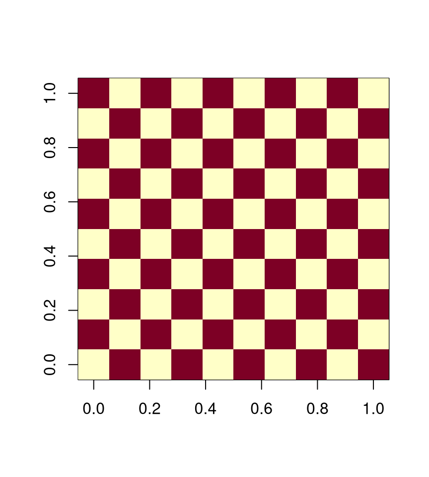
with \(\mathcal{C}_1 = \text{red}\) and \(\mathcal{C}_2 = \text{white}\)

For an 8-neighbor lattice four groups are needed.

Each group can be updated as a group, either

• using vectorized arithmetic, or
• using parallel computation

A vectorized implementation based on this approach:

nn <- function(m, c) {
    nr <- nrow(m)
    nc <- ncol(m)
    nn <- matrix(0, nr, nc)
    nn[1:(nr)-1,] <- nn[1:(nr)-1,] + (m[2:nr,] == c)
    nn[2:nr,] <- nn[2:nr,] + (m[1:(nr-1),] == c)
    nn[,1:(nc)-1] <- nn[,1:(nc)-1] + (m[,2:nc] == c)
    nn[,2:nc] <- nn[,2:nc] + (m[,1:(nc-1)] == c)
    nn
}

simGroup <- function(m, l2, l1, beta, which) {
    pp2 <- l2 * exp(beta * nn(m, 2))
    pp1 <- l1 * exp(beta * nn(m, 1))
    pp <- pp2 / (pp2 + pp1)
    ifelse(runif(sum(which)) < pp[which], 2, 1)
}

simImgV <- function(m, img, N, beta, p) {
    white <- outer(1:nrow(m), 1:ncol(m), FUN=`+`) %% 2 == 1
    black <- ! white
    if (is.null(img)) {
        l2 <- 1
        l1 <- 1
    }
    else {
        l2 <- ifelse(img == 2, p, 1 - p)
        l1 <- ifelse(img == 1, p, 1 - p)
    }
    for (i in 1:N) {
    m[white] <- simGroup(m, l2, l1, beta, white)
    m[black] <- simGroup(m, l2, l1, beta, black)
    }
    m
}

The results:

system.time(simImgV(m, img, 100, .35, .7))
##    user  system elapsed 
##   0.083   0.000   0.084

10.5 More MCMC Examples

10.5.1 Monte Carlo Maximum Likelihood

Suppose we have an exponential family likelihood

\[\begin{equation*} h(x|\theta) = c(\theta) e^{\theta x - \nu(x)} = c(\theta) \tilde{h}(x|\theta) \end{equation*}\]

In many problems \(c(\theta)\) is not available in closed form:

• Strauss process with \(\theta = \log c\).
• MRF image model with \(\theta = \beta\).

Geyer and Thompson (1992) write

\[\begin{equation*} \log\frac{h(x|\theta)}{h(x|\eta)} = \log\frac{\tilde{h}(x|\theta)}{\tilde{h}(x|\eta)} - \log E_\eta\left[\frac{\tilde{h}(X|\theta)}{\tilde{h}(X|\eta)}\right] \end{equation*}\]

This follows from the fact that

\[\begin{equation*} \frac{c(\theta)}{c(\eta)} = \frac{1}{c(\eta) \int\tilde{h}(x|\theta) dx} = \left(\int\frac{\tilde{h}(x|\theta)}{\tilde{h}(x|\eta)} c(\eta)\tilde{h}(x|\eta)dx\right)^{-1} = \left(E_\eta\left[\frac{\tilde{h}(X|\theta)}{\tilde{h}(X|\eta)} \right]\right)^{-1} \end{equation*}\]

Using a sample \(x_1, \dots, x_N\) from \(h(x|\eta)\) this can be approximated by

\[\begin{equation*} \log\frac{h(x|\theta)}{h(x|\eta)} \approx \log\frac{\tilde{h}(x|\theta)}{\tilde{h}(x|\eta)} - \log \frac{1}{N} \sum_{i=1}^N \frac{\tilde{h}(x_i|\theta)}{\tilde{h}(x_i|\eta)} \end{equation*}\]

The sample \(x_1, \dots, x_N\) from \(h(x|\eta)\) usually needs to be generated using MCMC methods.

10.5.2 Data Augmentation

Suppose we have a problem where data \(Y, Z\) have joint density \(f(y,z|\theta)\) but we only observe \(z\).

Suppose we have a prior density \(f(\theta)\).

The joint density of \(Y,Z,\theta\) is then

\[\begin{equation*} f(y,z,\theta) = f(y, z|\theta) f(\theta) \end{equation*}\]

and the joint posterior density of \(\theta, y\) given \(z\) is

\[\begin{equation*} f(\theta, y|z) = \frac{f(y, z|\theta) f(\theta)}{f(z)} \propto f(y, z|\theta) f(\theta) \end{equation*}\]

Suppose it is easy to sample from the conditional distribution of

• the missing data \(y\), given \(\theta\) and the observed data \(z\);
• the parameter \(\theta\) given the complete data \(y, z\).

Then we can start with \(\theta^{(0)}\) and for each \(i=1, 2, \dots\)

• draw \(y^{(i)}\) from \(f(y|\theta^{(i-1)}, z)\);
• draw \(\theta^{(i)}\) from \(f(\theta|y^{(i)},z)\).

This is the data augmentation algorithm of Tanner and Wong (1987)

The result is a Markov chain with stationary distribution \(f(\theta,y|z)\)

If we discard the \(y\) values then we have a (dependent) sample from the marginal posterior density \(f(\theta|z)\).

In this alternating setting, the marginal sequence \(\theta^{(i)}\) is a realization of a Markov chain with invariant distribution \(f(\theta|z)\).

10.5.3 Probit Model for Pesticide Effectiveness

Batches of 20 tobacco budworms were subjected to different doses of a pesticide and the number killed was recorded.

Dose	Died
1	1
2	4
4	9
8	13
16	18
32	20

A probit model assumes that binary responses \(Z_i\) depend on covariate values \(x_i\) though the relationship

\[\begin{equation*} Z_i \sim \text{Bernoulli}(\Phi(\alpha+\beta (x_i - \overline{x}))) \end{equation*}\]

A direct likelihood or Bayesian analysis is possible.

An alternative is to assume that there are latent variables \(Y_i\) with

\[\begin{align*} Y_i &\sim \text{N}(\alpha + \beta (x_i - \overline{x}), 1)\\ Z_i &= \begin{cases} 1 & \text{if $Y_i \ge 0$}\\ 0 & \text{if $Y_i < 0$} \end{cases} \end{align*}\]

For this example assume a flat, improper, prior density.

The full data posterior distribution is

\[\begin{equation*} f(\alpha,\beta|y) \propto \exp\left\{- \frac{n}{2} (\alpha - \overline{y})^2 - \frac{\sum(x_i-\overline{x})^2}{2}(\beta - \widehat{\beta})^2\right\} \end{equation*}\]

with

\[\begin{equation*} \widehat{\beta} = \frac{\sum(x_i-\overline{x})y_i}{\sum(x_i-\overline{x})^2} \end{equation*}\]

So \(\alpha\), \(\beta\) are independent given \(y\) and \(x\), and

\[\begin{align*} \alpha|y,z &\sim \text{N}(\overline{y}, 1/n)\\ \beta|y,z &\sim \text{N}(\widehat{\beta}, 1/\sum(x_i-\overline{x})^2) \end{align*}\]

Given \(z\), \(\alpha\), and \(\beta\) the \(Y_i\) are conditionally independent, and

\[\begin{equation*} Y_i|z, \alpha, \beta \sim \begin{cases} \text{N$(\alpha+\beta (x_i-\overline{x})^2,1)$ conditioned to be positive} & \text{if $z_i = 1$}\\ \text{N$(\alpha+\beta (x_i-\overline{x})^2,1)$ conditioned to be negative} & \text{if $z_i = 0$} \end{cases} \end{equation*}\]

The inverse CDF’s are

\[\begin{equation*} F^-(u|z_i,\mu_i) = \begin{cases} \mu_i + \Phi^{-1}(\Phi(-\mu_i) + u(1-\Phi(-\mu_i))) & \text{if $z_i = 1$}\\ \mu_i + \Phi^{-1}(u\,\Phi(-\mu_i)) & \text{if $z_i = 0$} \end{cases} \end{equation*}\]

with \(\mu_i = \alpha + \beta(x_i-\overline{x})\).

A plot of the proportion killed against dose is curved, but a plot against the logarithm is straight in the middle. So use \(x = \log_2(\text{dose})\).

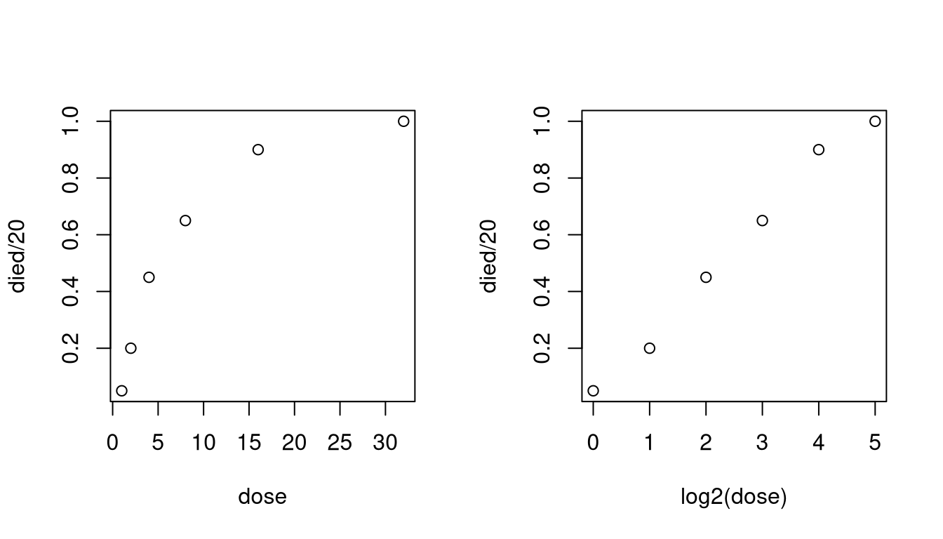
dose <- c(1, 2, 4, 8, 16, 32)
died <- c(1, 4, 9, 13, 18, 20)
x <- log2(dose)

We need to generate data for individual cases:

xx <- rep(x - mean(x), each = 20)
z <- unlist(lapply(died,
                   function(x) c(rep(1, x), rep(0, 20 - x))))

We need functions to generate from the conditional distributions:

genAlpha <- function(y)
    rnorm(1, mean(y), 1 / sqrt(length(y)))
genBeta <- function(y, xx, sxx2)
    rnorm(1, sum(xx * y) / sxx2, 1 / sqrt(sxx2))
genY <- function(z, mu) {
    p <- pnorm(-mu)
    u <- runif(length(z))
    mu + qnorm(ifelse(z == 1, p + u * (1 - p), u * p))
}

A function to produce a sample of parameter values by data augmentation is then defined by

da <- function(z, alpha, beta, xx, N) {
    val <- matrix(0, nrow = N, ncol = 2)
    colnames(val) <- c("alpha", "beta")
    sxx2 <- sum(xx^2)
    for (i in 1 : N) {
        y <- genY(z, alpha + beta * xx)
        alpha <- genAlpha(y)
        beta <- genBeta(y, xx, sxx2)
        val[i,1] <- alpha
        val[i,2] <- beta
    }
    val
}

Initial values are

alpha0 <- qnorm(mean(z))
beta0 <- 0

A run of 10000:

v <- da(z, alpha0, beta0, xx, 10000)
apply(v,2,mean)
##     alpha      beta 
## 0.2015720 0.7540646
apply(v,2,sd)
##     alpha      beta 
## 0.1480918 0.1140951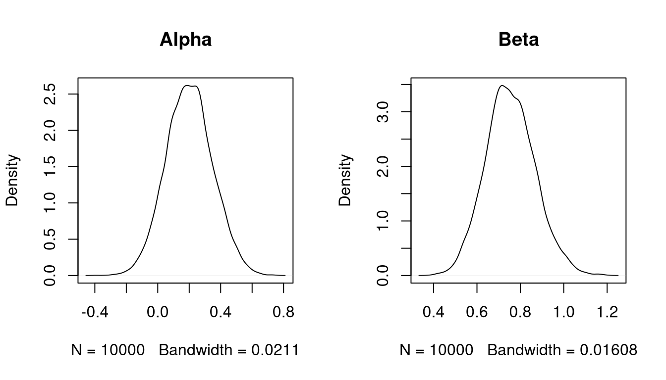

Some diagnostics:

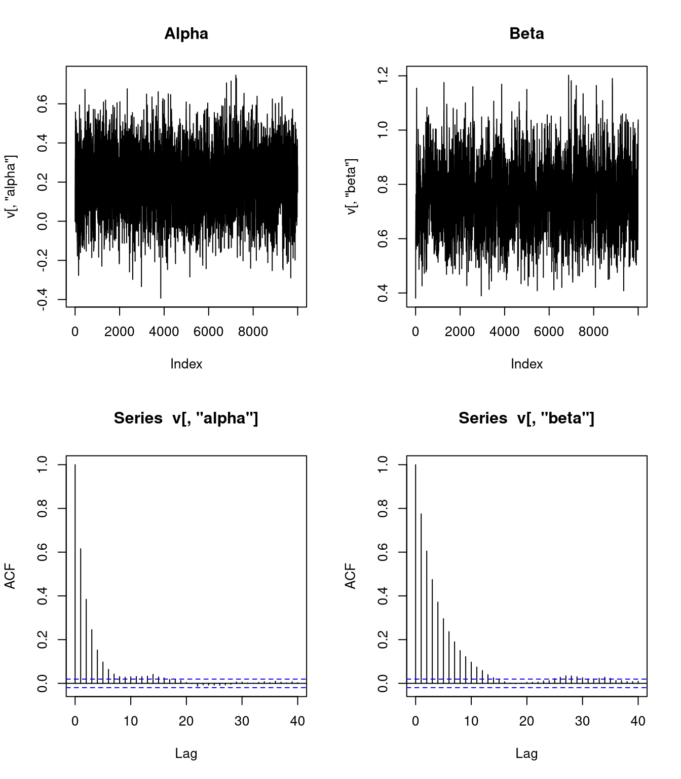
Using a simple AR(1) model,

\[\begin{align*} \text{SD}(\overline{\alpha}) &\approx \frac{\text{SD}(\alpha|z)}{\sqrt{N}} \sqrt{\frac{1+\rho_\alpha}{1-\rho_\alpha}} = \frac{0.1480918}{100}\sqrt{\frac{1+0.65}{1-0.65}} = 0.0032154\\ \text{SD}(\overline{\beta}) &\approx \frac{\text{SD}(\beta|z)}{\sqrt{N}} \sqrt{\frac{1+\rho_\beta}{1-\rho_\beta}} = \frac{0.1140951}{100}\sqrt{\frac{1+0.8}{1-0.8}} = 0.0034229 \end{align*}\]

Suppose we could sample independently from the posterior distribution. The number of independent draws needed to achieve the standard error \(\text{SD}(\overline{\alpha})\) is the value of \(N_E\) that solves the equation

\[\begin{equation*} \text{SD}(\overline{\alpha}) = \frac{\text{SD}(\alpha|z)}{\sqrt{N_E}}. \end{equation*}\]

This is the effective sample size \(\text{ESS}(\overline{\alpha})\).

The approximate effective sample sizes are

\[\begin{align*} \text{ESS}(\overline{\alpha}) &\approx N \left(\frac{1-\rho_\alpha}{1+\rho_\alpha}\right) = 10000 \left(\frac{1-0.65}{1+0.65}\right) = 2121.212\\ \text{ESS}(\overline{\beta}) &\approx N \left(\frac{1-\rho_\beta}{1+\rho_\beta}\right) = 10000 \left(\frac{1-0.8}{1+0.8}\right) = 1111.111\\ \end{align*}\]

Approximate efficiencies:

\[\begin{align*} \text{Efficiency}(\overline{\alpha}) = \frac{\text{ESS}(\overline{\alpha})}{N} &\approx \left(\frac{1-\rho_\alpha}{1+\rho_\alpha}\right) = \left(\frac{1-0.65}{1+0.65}\right) = 0.2121\\ \text{Efficiency}(\overline{\beta}) = \frac{\text{ESS}(\overline{\beta})}{N} &\approx \left(\frac{1-\rho_\beta}{1+\rho_\beta}\right) = \left(\frac{1-0.8}{1+0.8}\right) = 0.1111\\ \end{align*}\]

10.6 Practical Bayesian Inference

In Bayesian inference we have

• a prior density or PMF \(f(\theta)\);
• a data density or PMF, or likelihood, \(f(x|\theta)\).

We compute the posterior density or PMF as

\[\begin{equation*} f(\theta|x) = \frac{f(x|\theta)f(\theta)}{f(x)} \propto f(x|\theta)f(\theta). \end{equation*}\] At this point, in principle, we are done.

In practice, if \(\theta = (\theta_1,\dots,\theta_p)\) then we want to compute things like

• the posterior means \(E[\theta_i|x]\) and variances \(\text{Var}(\theta_i|x)\);
• the marginal posterior densities \(f(\theta_i|x)\);
• posterior probabilities, such as \(P(\theta_1 > \theta_2|x)\).

These are all integration problems.

For a few limited likelihood/prior combinations we can compute these integrals analytically.

For most reasonable likelihood/prior combinations analytic computation is impossible.

10.6.1 Numerical Integration

For \(p = 1\)

• we can plot the posterior density;
• we can compute means and probabilities by numerical integration.

General one dimensional numerical integration methods like

• the trapezoidal rule;
• Simpson’s rule;
• adaptive methods (as in integrate in R).

often use \(N \approx 100\) function evaluations.

If \(p=2\) we can

• plot the joint posterior density;
• compute marginal posterior densities by one dimensional numerical integrations and plot them;
• compute means and probabilities by iterated one dimensional numerical integration.

In general, iterated numerical integration requires \(N^p\) function evaluations.

If a one dimensional \(f\) looks like

\[\begin{equation*} f(x) \approx (\text{ low degree polynomial}) \times (\text{normal density}) \end{equation*}\]

then Gaussian quadrature (Monahan, p. 268–271; Givens and Hoeting, Section 5.3) may work with \(N = 3\) or \(N = 4\).

• This approach is used in Naylor and Smith (1984).
• Getting the location and scale of the Gaussian right is critical.
• Even \(3^p\) gets very large very fast.

10.6.2 Large Sample Approximations

If the sample size \(n\) is large,

\[\begin{align*} \widehat{\theta}& = \text{mode of joint posterior density $f(\theta|x)$}\\ H &= - \nabla^2_\theta \; \log f(\widehat{\theta}|x)\\ &= \text{Hessian (matrix of second partial derivatives) of $-\log f$ at $\widehat{\theta}$} \end{align*}\]

then under often reasonable conditions

\[\begin{equation*} f(\theta|x) \approx \text{MVN}_p(\widehat{\theta},H^{-1}) \end{equation*}\]

The relative error in the density approximation is generally of order \(O(n^{-1/2})\) near the mode.

More accurate second order approximations based on Laplace’s method are also sometimes available.

To approximate the marginal posterior density of \(\theta_1\), compute

\[\begin{align*} \widehat{\theta}_2(\theta_1) &= \text{argmax}_{\theta_2} f(\theta_1,\theta_2|x)\\ H(\theta_1) &= - \nabla^2_{\theta_2} \; \log f(\theta_1,\widehat{\theta}_2(\theta_1)|x) \end{align*}\]

Then

\[\begin{equation*} \hat{f}(\theta_1|x) \propto \sqrt{\det H(\theta_1)} f(\theta_1,\widehat{\theta}_2(\theta_1)|x) \end{equation*}\]

approximates \(f(\theta_1|x)\) with a relative error near the mode of order \(O(n^{-3/2})\).

The component \(f(\theta_1,\widehat{\theta}_2(\theta_1)|x)\) is analogous to the profile likelihood.

The term \(\sqrt{\det H(\theta_1)}\) adjusts for differences in spread in the parameter being maximized out.

10.6.3 Monte Carlo Methods

Early Monte Carlo approaches used importance sampling.

• Usually some form of multivariate \(t\) is used to get heavy tails and bounded weights.
• Guaranteeing bounded weights in high dimensions is very hard.
• Even bounded weights may have too much variation to behave well.

Tanner and Wong (1987) introduced the idea of Markov chain sampling for data augmentation.

Gelfand and Smith (1989) showed that many joint posterior distributions have simple full conditional distributions

\[\begin{equation*} f(\theta_i|x, \theta_1,\dots,\theta_{i-1},\theta_{i+1},\dots,\theta_p) \end{equation*}\]

These can be sampled using a Markov chain, called a Gibbs sampler.

The systematic scan Gibbs sampler starts with some initial values \(\theta_1^{(0)},\dots,\theta_p^{(0)}\) and then for each \(k\) generates

\[\begin{align*} \theta_1^{(k+1)} &\sim f(\theta_1|x, \theta_2=\theta_2^{(k)},\dots,\theta_p = \theta_p^{(k)})\\ &\;\;\vdots\\ \theta_i^{(k+1)} &\sim f(\theta_i|x, \theta_1=\theta_1^{(k+1)},\dots, \theta_{i-1}=\theta_{i-1}^{(k+1)}, \theta_{i+1}=\theta_{i+1}^{(k)},\dots, \theta_p = \theta_p^{(k)})\\ &\;\;\vdots\\ \theta_p^{(k+1)} &\sim f(\theta_p|x, \theta_1=\theta_1^{(k+1)},\dots, \theta_{p-1} = \theta_{p-1}^{(k+1)})\\ \end{align*}\]

The random scan Gibbs sampler picks an index \(i=1,\dots,p\) at random and updates that component from its full conditional distribution.

The random scan Gibbs sampler is the approach proposed by Ripley (1979).

Many other variations are possible.

All generate a Markov chain \(\theta^{(0)}, \theta^{(1)}, \theta^{(2)},\dots,\) with invariant distribution \(f(\theta|x)\).

10.6.4 Example: Pump Failure Data

Numbers of failures and times of observation for 10 pumps in a nuclear power plant:

Pump	1	2	3	4	5	6	7	8	9	10
Failures	5	1	5	14	3	19	1	1	4	22
Time	94.32	15.72	62.88	125.76	5.24	31.44	1.05	1.05	2.10	10.48

Times are in 1000’s of hours.

Suppose the failures follow Poisson processes with rates \(\lambda_i\) for pump \(i\); so the number of failures on pump \(i\) is \(X_i \sim \text{Poisson}(\lambda_i t_i)\).

The rates \(\lambda_i\) are drawn from a \(\text{Gamma}(\alpha,1/\beta)\) distribution.

Assume \(\alpha = 1.8\)

Assume \(\beta \sim \text{Gamma}(\gamma, 1/\delta)\) with \(\gamma = 0.01\) and \(\delta = 1\).

The joint posterior distribution of \(\lambda_1,\dots,\lambda_{10},\beta\) is

\[\begin{align*} f(\lambda_1,\dots,\lambda_{10},\beta|t_1,\dots,t_{10},x_1,\dots,x_{10}) &\propto \left(\prod_{i=1}^{10}(\lambda_i t_i)^{x_i} e^{-\lambda_i t_i} \lambda_i^{\alpha-1}\beta^\alpha e^{-\beta\lambda_i}\right) \beta^{\gamma-1}e^{-\delta\beta}\\ &\propto \left(\prod_{i=1}^{10}\lambda_i^{x_i+\alpha-1} e^{-\lambda_i(t_i + \beta)}\right) \beta^{10\alpha + \gamma-1}e^{-\delta\beta}\\ &\propto \left(\prod_{i=1}^{10}\lambda_i^{x_i+\alpha-1} e^{-\lambda_i t_i}\right) \beta^{10\alpha + \gamma-1}e^{-(\delta + \sum_{i=1}^{10}\lambda_i)\beta} \end{align*}\]

Full conditionals:

\[\begin{align*} \lambda_i | \beta, t_i, x_i &\sim \text{Gamma}(x_i+\alpha,(t_i+\beta)^{-1})\\ \beta | \lambda_i, t_i, x_i &\sim \text{Gamma}(10\alpha+\gamma,(\delta+\sum \lambda_i)^{-1}) \end{align*}\]

It is also possible to integrate out the \(\lambda_i\) analytically to get

\[\begin{equation*} f(\beta|t_i,x_i) \propto \left(\prod_{i=1}^{10}(t_i+\beta)^{x_i+\alpha} \right)^{-1} \beta^{10\alpha + \gamma-1}e^{-\delta\beta} \end{equation*}\]

This can be simulated by rejection or RU sampling; the \(\lambda_i\) can then be sampled conditionally given \(\beta\).

Suppose \(\alpha\) is also unknown and given an exponential prior distribution with mean one.

The joint posterior distribution is then

\[\begin{equation*} f(\lambda_1,\dots,\lambda_{10},\beta, \alpha|t_i, x_i) \propto \left(\prod_{i=1}^{10}\lambda_i^{x_i+\alpha-1} e^{-\lambda_i(t_i + \beta)}\right) \beta^{10\alpha + \gamma-1}e^{-\delta\beta} \frac{e^{-\alpha}}{\Gamma(\alpha)^{10}} \end{equation*}\]

The full conditional density for \(\alpha\) is

\[\begin{equation*} f(\alpha|\beta, \lambda_i, t_i, x_i) \propto \frac{\left(\beta^{10}e^{-1}\prod_{i=1}^{10}\lambda_i\right)^\alpha} {\Gamma(\alpha)^{10}} \end{equation*}\]

This is not a standard density

This density is log-concave and can be sampled by adaptive rejection sampling.

Another option is to use the Metropolis-Hastings algorithm.

10.7 Metropolis-Hasting Algorithm

Introduced in N, Metropolis, A. W. Rosenbluth, M. N. Rosenbluth, A. H. Teller, and E. Teller (1953), “Equations for state space calculations by fast computing machines,” Journal of Chemical Physics.

Extended in Hastings (1970), “Monte Carlo sampling methods using Markov chains and their applications,” Biometrika.

Suppose we want to sample from a density \(f\).

We need a family of proposal distributions \(Q(x,dy)\) with densities \(q(x,y)\).

Suppose a Markov chain with stationary distribution \(f\) is currently at \(X^{(i)} = x\). Then

• Generate a proposal \(Y\) for the new location by drawing from the density \(q(x,y)\).
• Accept the proposal with probability \[\begin{equation*} \alpha(x,y) = \min\left\{\frac{f(y)q(y,x)}{f(x)q(x,y)}, 1\right\} \end{equation*}\] and set \(X^{(i+1)} = Y\).
• Otherwise, reject the proposal and remain at \(x\), i.e. set \(X^{(i+1)} = x\).

The resulting transition densities satisfy the detailed balance equations for \(x \neq y\) and initial distribution \(f\):

\[\begin{equation*} f(x) q(x,y) \alpha(x,y) = f(y) q(y,x) \alpha(y,x) \end{equation*}\]

The chain is therefore reversible and has invariant distribution \(f\).

10.7.1 Symmetric Proposals

Suppose \(q(x,y) = q(y,x)\). Then

\[\begin{equation*} \alpha(x,y) = \min\left\{\frac{f(y)}{f(x)},1\right\} \end{equation*}\] So:

• If \(f(y) \ge f(x)\) then the proposal is accepted.
• If \(f(y) < f(x)\) then the proposal is accepted with probability \[\begin{equation*} \alpha(x,y) = \frac{f(y)}{f(x)} < 1 \end{equation*}\]

Symmetric proposals are often used in the simulated annealing optimization method.

Symmetric random walk proposals with \(q(x, y) = g(y-x)\) where \(g\) is a symmetric density are often used.

Metropolis et al. (1953) considered only the symmetric proposal case.

Hastings (1970) introduced the more general approach allowing for non-symmetric proposals.

10.7.2 Independence Proposals

Suppose \(q(x,y) = g(y)\), independent of \(x\). Then

\[\begin{equation*} \alpha(x,y) = \min\left\{\frac{f(y)g(x)}{f(x)g(y)}, 1\right\} = \min\left\{\frac{w(y)}{w(x)}, 1\right\} \end{equation*}\]

with \(w(x) = f(x)/g(x)\).

This is related to importance sampling:

• If a proposal \(y\) satisfies \(w(y) \ge w(x)\) then the proposal is accepted.
• If \(w(y) < w(x)\) then the proposal may be rejected.
• If the weight \(w(x)\) at the current location is very large, meaning \(g(x)\) is very small compared to \(f(x)\), then the chain will remain at \(x\) for many steps to compensate.

10.7.3 Metropolized Rejection Sampling

Suppose \(h(x)\) is a possible envelope for \(f\) with \(\int h(x) dx < \infty\).

Suppose we sample

• \(Y\) from \(h\)
• \(U\) uniformly on \([0,h(Y)]\)

until \(U < f(Y)\).

Then the resulting \(Y\) has density

\[\begin{equation*} g(y) \propto \min(h(x),f(x)) \end{equation*}\]

Using \(g\) as a proposal distribution, the Metropolis acceptance probability is

\[\begin{align*} \alpha(x,y) &=\min\left\{\frac{f(y)\min(h(x),f(x))}{f(x)\min(h(y),f(y))}, 1\right\}\\ &= \min\left\{\frac{\min(h(x)/f(x), 1)}{\min(h(y)/f(y),1)},1\right\}\\ &= \begin{cases} 1 & \text{if $f(x) \le h(x)$}\\ h(x)/f(x) & \text{if $f(x) > h(x)$ and $f(y) \le h(y)$}\\ \min\left\{\frac{f(y)h(x)}{f(x)h(y)},1\right\} &\text{otherwise} \end{cases}\\ &= \min\left\{\frac{h(x)}{f(x)}, 1\right\} \min\left\{\max\left\{\frac{f(y)}{h(y)},1\right\}, \max\left\{\frac{f(x)}{h(x)},1\right\}\right\}\\ & \ge \min\left\{\frac{h(x)}{f(x)}, 1\right\} \end{align*}\]

If \(h\) is in fact an envelope for \(f\), then \(\alpha(x,y) \equiv 1\) and the algorithm produces independent draws from \(f\).

If \(h\) is not an envelope, then the algorithm occasionally rejects proposals when the chain is at points \(x\) where the envelope fails to hold.

The dependence can be very mild if the failure is mild; it can be very strong if the failure is significant.

10.7.4 Metropolis-Within-Gibbs

Suppose \(f(x) = f(x_1, \dots, x_p)\)

The Metropolis-Hastings algorithm can be used on the entire vector \(x\).

The Metropolis-Hastings algorithm can also be applied to one component of a vector using the full conditional density

\[\begin{equation*} f(x_i|x_1,\dots,x_{i-1},x_{i+1},\dots,x_p) \end{equation*}\]

as the target density.

This approach is sometimes called Metropolis-within-Gibbs.

This is a misnomer: this is what Metropolis et al. (1953) did to sample from the equilibrium distribution of \(n\) gas molecules.

10.7.5 Example: Pump Failure Data

Suppose \(\alpha\) has an exponential prior distribution with mean 1.

The full conditional density for \(\alpha\) is

\[\begin{equation*} f(\alpha|\beta, \lambda_i, t_i, x_i) \propto \frac{\left(\beta^{10}e^{-1}\prod_{i=1}^{10}\lambda_i\right)^\alpha} {\Gamma(\alpha)^{10}} \end{equation*}\]

To use a random walk proposal it is useful to make the support of the distribution be the whole real line.

The full conditional density of \(\log \alpha\) is

\[\begin{equation*} f(\log \alpha|\beta, \lambda_i, t_i, x_i) \propto \frac{\left(\beta^{10}e^{-1}\prod_{i=1}^{10}\lambda_i\right)^\alpha\alpha} {\Gamma(\alpha)^{10}} \end{equation*}\]

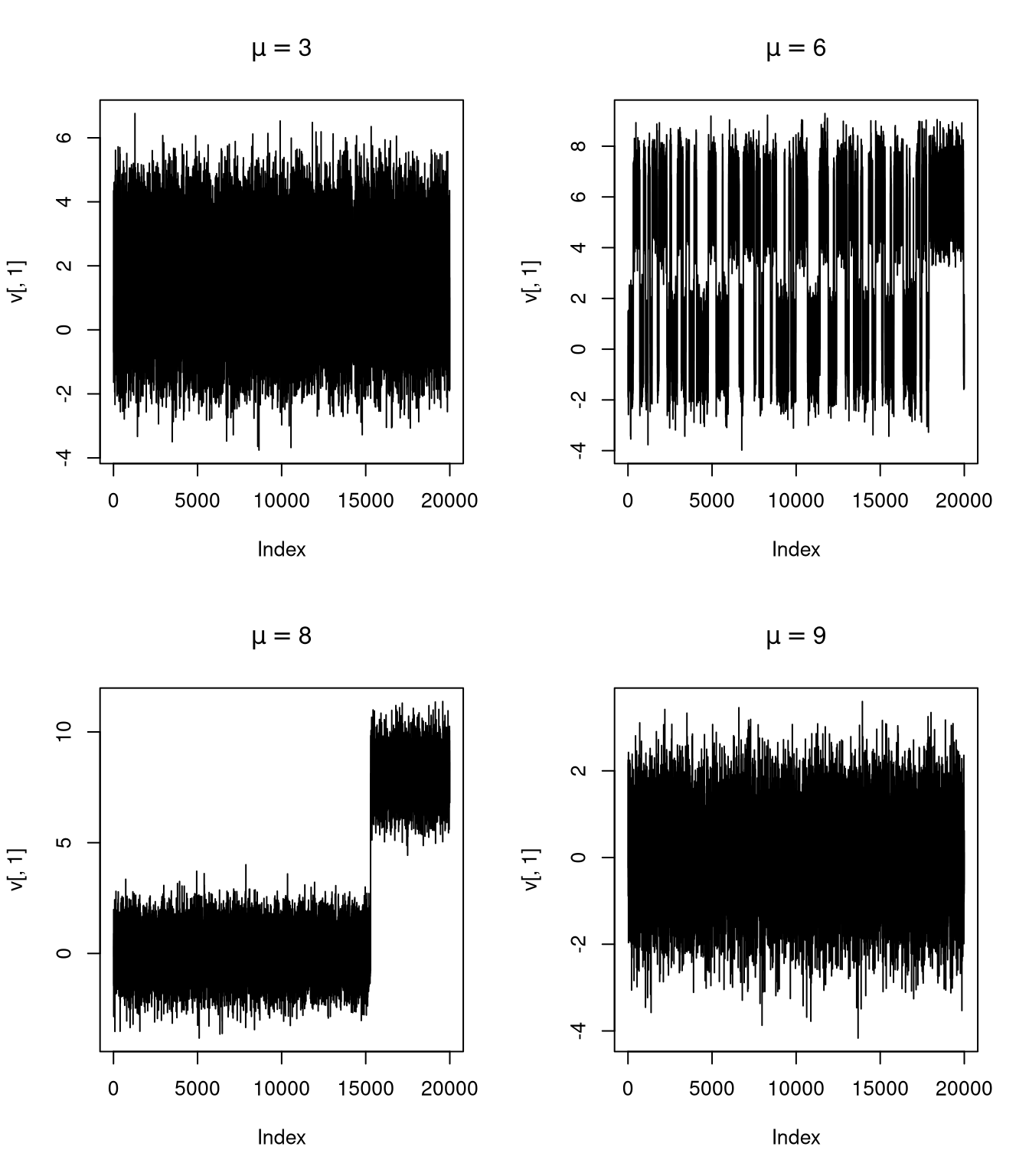
Using a normal random walk proposal requires choosing a standard deviation; 0.7 seems to work reasonably well.

We can use a single Metropolis step or several.

10.7.6 Gibbs Sampler in R for Pump Data

The data:

fail <- c(5, 1, 5, 14, 3, 19, 1, 1, 4, 22)
time <- c(94.32, 15.72, 62.88, 125.76, 5.24,
          31.44, 1.05, 1.05, 2.10, 10.48)

Hyper-parameters for the prior distribution:

alpha <- 1.8
gamma <- 0.01
delta <- 1

Generator for the full conditional for \(\lambda_i, i = 1, \dots, 10\):

genLambda <- function(alpha, beta)
    rgamma(10, fail + alpha, rate = time + beta)

Generator for the full conditional for \(\beta\):

genBeta <- function(alpha, lambda)
    rgamma(1, 10 * alpha + gamma, rate = delta + sum(lambda))

Metropolis-Hastings sampler for the full conditional for \(\alpha\) (for \(K = 0\) the value of \(\alpha\) is unchanged):

genAlpha <- function(alpha, beta, lambda, K, d) {
    b <- (10 * log(beta) + sum(log(lambda)) - 1)
    for (j in seq_len(K)) {
        newAlpha <- exp(rnorm(1, log(alpha), d))
        logDensRatio <-
            ((newAlpha - alpha) * b +
             log(newAlpha) - log(alpha) +
             10 * (lgamma(alpha) - lgamma(newAlpha)))
        if (is.finite(logDensRatio) &&
            log(runif(1)) < logDensRatio)
            alpha <- newAlpha
    }
    alpha
}

Driver for running the sampler:

pump <- function(alpha, beta, N, d = 1, K = 1) {
    v <- matrix(0, ncol=12, nrow=N)
    for (i in 1:N) {
        lambda <- genLambda(alpha, beta)
        beta <- genBeta(alpha, lambda)
        alpha <- genAlpha(alpha, beta, lambda, K, d)
        v[i,1:10] <- lambda
        v[i,11] <- beta
        v[i,12] <- alpha
    }
    v
}

Run the sampler:

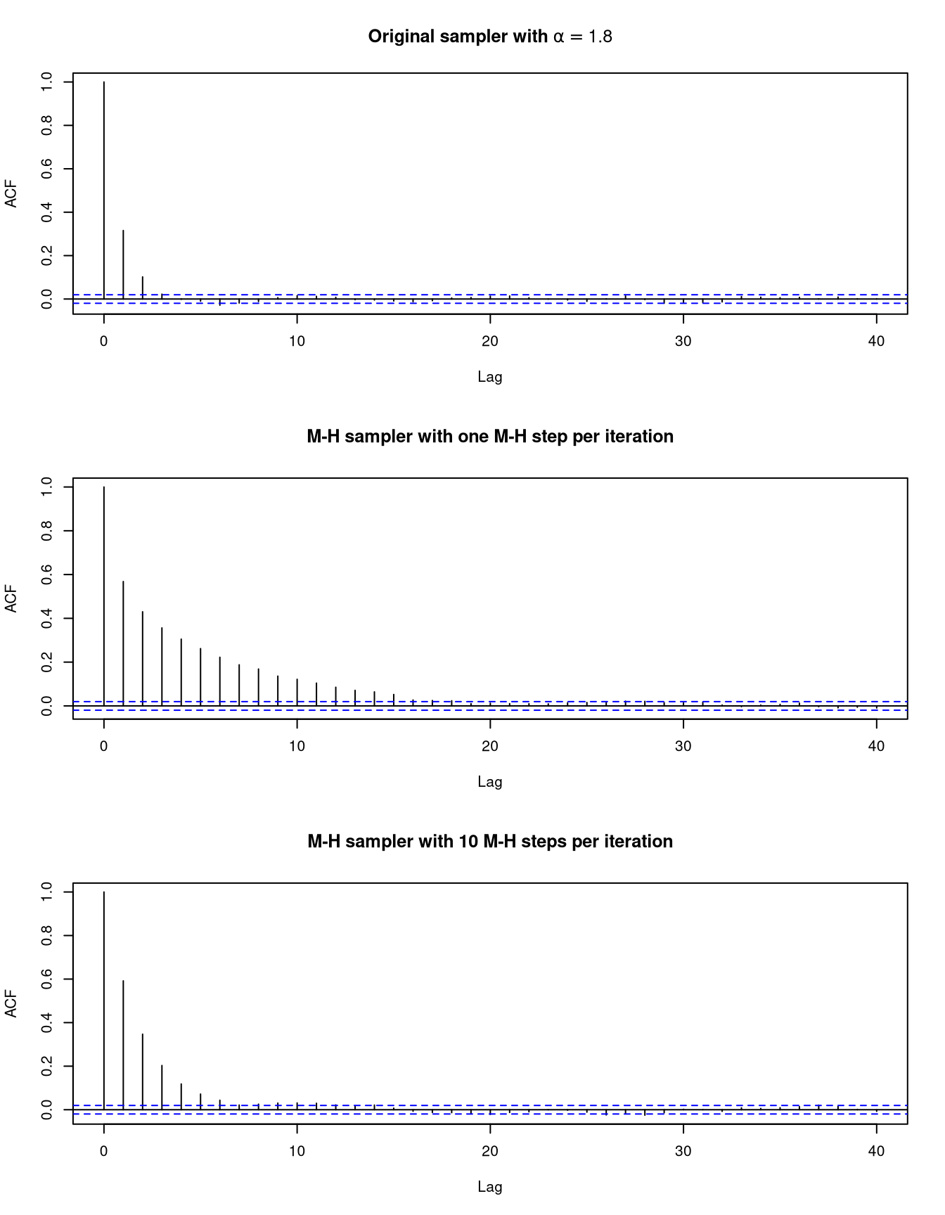
v0 <- pump(alpha, beta = 1, 10000, K = 0)
v1 <- pump(alpha, beta = 1, 10000, K = 1)
v10 <- pump(alpha, beta = 1, 10000, K = 10)

Marginal densities for \(\beta\) and joint marginal densities for \(\alpha\) and \(\beta\):

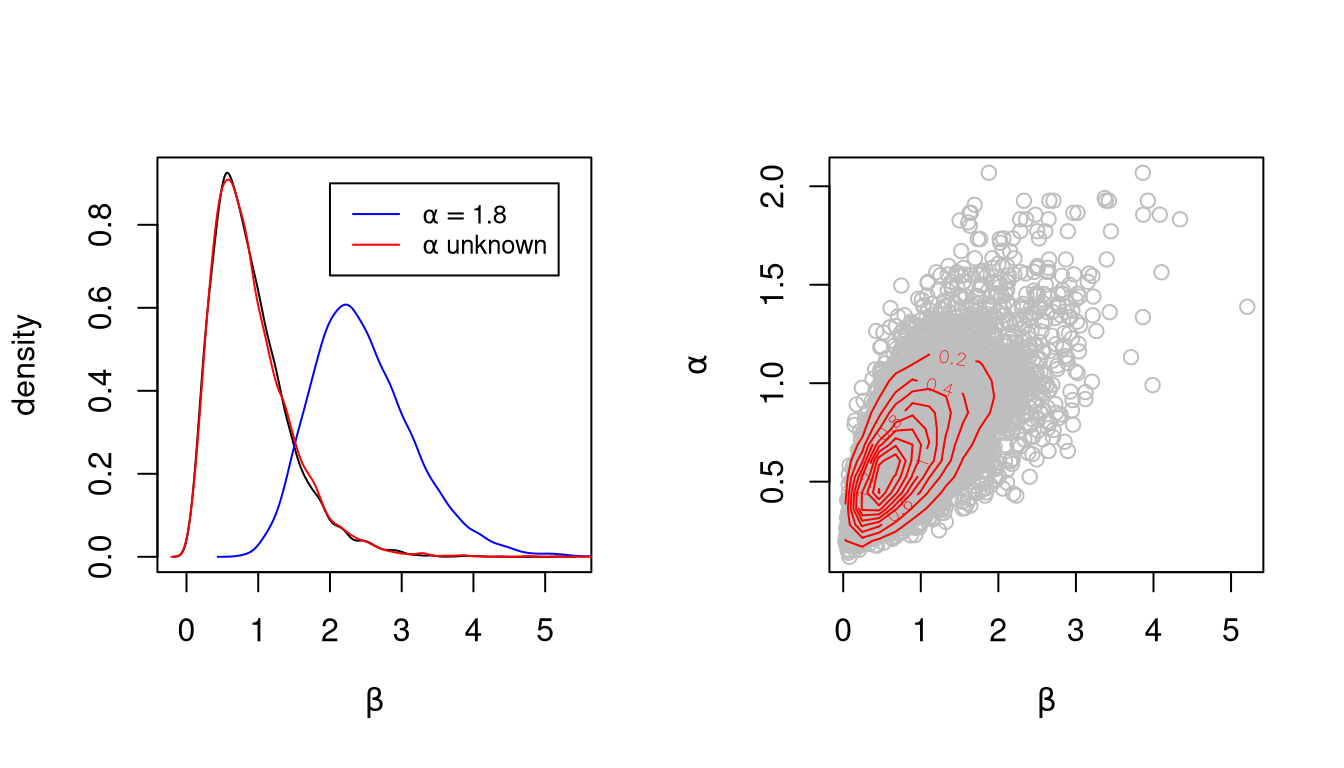
Auto-correlation functions for \(\beta\)

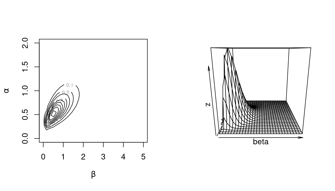
As an aside, is it possible in this case to integrate out the \(\lambda_i\) to obtain the joint marginal posterior density of \(\alpha\) and \(\beta\) as

\[\begin{equation*} f(\alpha, \beta | t_i, x_i) \propto \frac{\prod_{i=1}^{10} \Gamma(x_i + \alpha)} {\Gamma(\alpha)^{10}\prod_{i=1}^{10} (t_i + \beta)^{x_i + \alpha}} \beta^{10 \alpha + \gamma - 1} e^{-\delta\beta}e^{-\alpha} \end{equation*}\]

Plots of this joint distribution match the results of the simulation:

10.8 Markov Chain Theory: Discrete State Space

A sequence of random variables \(X_0, X_1, X_2, \dots\) with values in a finite or countable set \(E\) is a Markov chain if for all \(n\)

\[\begin{equation*} P(X_{n+1} = j|X_n=i, X_{n-1}, X_{n-2},\dots, X_0) = P(X_{n+1}=j|X_n=i) \end{equation*}\]

i.e. given the present, the future and the past are independent.

A Markov chain is time homogeneous if

\[\begin{equation*} P(i,j) = P(X_{n+1} = j|X_n=i) \end{equation*}\]

does not depend on \(n\). \(P(i,j)\) is the transition matrix of the Markov chain.

A transition matrix satisfies

\[\begin{equation*} \sum_{j \in E} P(i,j) = 1 \end{equation*}\]

for all \(i \in E\).

The distribution of \(X_0\) is called the initial distribution of a Markov chain.

The \(n\) step transition matrix is

\[\begin{equation*} P^n(i,j) = P(X_n=j|X_0=i) \end{equation*}\]

The \(n+m\) step transition matrix satisfies

\[\begin{equation*} P^{n+m} = P^n P^m \end{equation*}\]

That is,

\[\begin{equation*} P^{n+m}(i,j) = \sum_{k \in E} P^n(i,k)P^m(k,j) \end{equation*}\]

for all \(i, j \in E\).

A distribution \(\pi\) is an invariant distribution or a stationary distribution for a Markov transition matrix \(P\) if

\[\begin{equation*} \pi(j) = \sum_{i \in E} \pi(i) P(i,j) \end{equation*}\] for all \(i\). These equations are sometimes called the flow balance equations

10.8.1 Reversibility

A transition matrix is reversible with respect to a distribution \(\pi\) if

\[\begin{equation*} \pi(i) P(i,j) = \pi(j) P(j,i) \end{equation*}\]

for every pair \(i,j\). These equations are called the detailed balance equations.

If \(P\) is reversible with respect to \(\pi\), then \(\pi\) is a stationary distribution for \(P\):

\[\begin{equation*} \sum_{i \in E} \pi(i) P(i,j) = \sum_{i \in E} \pi(j) P(j,i) = \pi(j) \sum_{i \in E} P(j,i) = \pi(j) \end{equation*}\]

If \(P\) is reversible with respect to \(\pi\) and \(X_0\) has initial distribution \(\pi\), then the vectors

\[\begin{equation*} (X_0, X_1, X_2, \dots, X_{n-2}, X_{n-1}, X_n) \end{equation*}\]

and

\[\begin{equation*} (X_n, X_{n-1}, X_{n-2}, \dots, X_2, X_1, X_0) \end{equation*}\]

have the same joint distributions.

Reversible transition matrices have many nice properties, including real eigenvalues.

10.8.2 Convergence

A Markov chain is irreducible if for each pair of states \(i,j\) there is an integer \(n\) such that

\[\begin{equation*} P^n(i,j) > 0 \end{equation*}\]

i.e. if each state can be reached with positive probability from any other state.

The time to reach state \(i\) is

\[\begin{equation*} \tau_i = \min\{n \ge 1: X_n = i\} \end{equation*}\]

with \(\tau_i = \infty\) if \(X_n \neq i\) for all \(n\).

An irreducible Markov chain falls into one of three categories:

• Transient: \(P(\tau_i = \infty|X_0=j) > 0\) for all \(i,j \in E\).

• Null recurrent: \(P(\tau_i = \infty|X_0=j) = 0\) and \(E[\tau_i|X_0=j] = \infty\) for all \(i,j \in E\).

• Positive recurrent: \(P(\tau_i = \infty|X_0=j) = 0\) and \(E[\tau_i|X_0=j] < \infty\) for all \(i,j \in E\).

If an irreducible Markov chain is transient or null recurrent then it does not have a proper invariant distribution.

If an irreducible Markov chain is positive recurrent, then

• it has a unique invariant distribution \(\pi\);

• for any \(i \in E\) \[\begin{equation*} \frac{1}{n} \sum_{k=1}^n P^k(i,j) \to \pi(j); \end{equation*}\]

• if \(h\) is a real-valued function on \(E\) such that \[\begin{equation*} \sum_{i \in E} |h(i)| \pi(i) < \infty \end{equation*}\] then almost surely \[\begin{equation*} \frac{1}{n}\sum_{k=1}^n h(X_k) \to \pi h = \sum_{i \in E} h(i)\pi(i); \end{equation*}\]

• if the chain is also aperiodic, then \[\begin{equation*} P^n(i, j) = \to \pi(j) \end{equation*}\] for all \(i, j \in E\). In this case \(\pi\) is an equilibrium distribution of the chain.

10.8.3 Different Points of View

In applied probability problems we usually

• verify that a chain is irreducible;

• verify that a chain is positive recurrent;

• conclude that a unique stationary distribution exists;

• compute the unique stationary distribution \(\pi\);

• verify that the chain is aperiodic;

• use \(\pi\) to approximate the distribution of \(X_n\).

In Markov chain Monte Carlo

• we know by construction that a proper stationary distribution \(\pi\) exists;

• we verify that the chain is irreducible;

• we conclude that the chain must be positive recurrent (since it cannot be transient or null recurrent) and therefore \(\pi\) is the unique stationary distribution;

• we approximate expectations under \(\pi\) by sample path averages;

• aperiodicity is usually not important.

10.9 Markov Chain Theory: General State Spaces

Let \(E\) be an arbitrary set and \(\mathcal{E}\) a countably generated sigma-algebra on \(E\).

A sequence of \((E,\mathcal{E})\)-valued random variables is a time homogeneous Markov chain with transition kernel \(P(x,dy)\) if

\[\begin{equation*} P(X_{n+1} \in A|X_n, X_{n-1},\dots,X_0) = P(X_n, A) \end{equation*}\]

for all \(A \in \mathcal{E}\).

A Markov transition kernel is a function \(P(\cdot,\cdot)\) such that

• \(P(x,\cdot)\) is a probability on \((E,\mathcal{E})\) for each \(x \in E\).
• \(P(\cdot,A)\) is a \(\mathcal{E}\)-measurable function for each \(A \in \mathcal{E}\).

The \(n\)-step transition kernel of a Markov chain is

\[\begin{equation*} P^n(x,A) = P(X_n \in A| X_0 = x) \end{equation*}\]

and satisfies

\[\begin{equation*} P^{n+m}(x,A) = \int P^n(x,dy)P^m(y,A) \end{equation*}\]

for all \(x \in E\) and all \(A \in \mathcal{A}\).

A distribution \(\pi\) is invariant for a Markov transition kernel \(P\) if

\[\begin{equation*} \pi(A) = \int \pi(dy) P(y, A) \end{equation*}\] for all \(A \in \mathcal{E}\).

10.9.1 Reversibility

A transition kernel \(P\) is reversible with respect to a distribution \(\pi\) if

\[\begin{equation*} \pi(dx)P(x,dy) = \pi(dy)P(y,dx) \end{equation*}\]

i.e. these two bivariate distributions must be identical.

If \(P\) is reversible with respect to \(\pi\) then \(P\) is invariant with respect to \(\pi\):

\[\begin{align*} \int_{x \in E} \pi(dx) P(x,A) &= \int_{x \in E}\int_{y \in A} \pi(dx) P(x,dy)\\ &= \int_{x \in E}\int_{y \in A} \pi(dy) P(y,dx)\\ &= \int_{y \in A} \pi(dy) \int_{x \in E}P(y,dx)\\ &= \int_{y \in A} \pi(dy)\\ &= \pi(A) \end{align*}\]

10.9.2 Convergence

A Markov chain with transition kernel \(P\) is irreducible with respect to a sigma-finite measure \(\nu\) if for every \(x \in E\) and every \(A \in \mathcal{E}\) with \(\nu(A) > 0\) there exists an integer \(n\) such that \(P^n(x, A) > 0\)

A Markov chain is irreducible if it is irreducible with respect to \(\nu\) for some sigma-finite \(\nu\).

The standard definition of irreducibility for discrete state spaces corresponds to irreducibility with respect to counting measure for general state spaces.

An irreducible Markov chain is either transient, null recurrent, or positive recurrent.

An irreducible Markov chain is positive recurrent if and only if it has a proper stationary distribution \(\pi\).

Essentially all Markov chains used in MCMC that are recurrent are also Harris recurrent.

If an irreducible Markov chain is positive recurrent, then

• it has a unique stationary distribution \(\pi\)
• if the chain is Harris recurrent, then \[\begin{equation*} \sup_{A \in \mathcal{E}} \left|\frac{1}{n}\sum_{k=1}^nP^k(x,A)-\pi(A)\right| \to 0 \end{equation*}\] for all \(x\)
• if the chain is Harris recurrent, \(h\) is real-valued, \(\mathcal{E}\)-measurable, and \(\pi|h| = \int |h(x)|\pi(dx) < \infty\), then for any initial distribution \[\begin{equation*} \frac{1}{n} \sum_{k=1}^n h(X_k) \to \pi h = \int h(x) \pi(dx) \end{equation*}\]
• if the chain is Harris recurrent and aperiodic, then \[\begin{equation*} \sup_{A \in \mathcal{E}}|P^n(x,A)-\pi(A)| \to 0 \end{equation*}\] for all \(x\).

10.9.3 Rates of Convergence

A Markov chain is geometrically ergodic if there exists a nonnegative function \(M(x)\) with \(\pi M < \infty\) and a constant \(\lambda < 1\) such that

\[\begin{equation*} \sup_{A \in \mathcal{E}} |P^n(x,A)-\pi(A)| \le M(x)\lambda^n \end{equation*}\]

for all \(x \in E\) and all integers \(n \ge 1\).

A Markov chain is uniformly ergodic if there exists a finite constant \(M\) and a constant \(\lambda < 1\) such that

\[\begin{equation*} \sup_{A \in \mathcal{E}} |P^n(x,A)-\pi(A)| \le M\lambda^n \end{equation*}\]

for all \(x \in E\) and all integers \(n \ge 1\).

Many MCMC samplers are geometrically ergodic; relatively few are uniformly ergodic.

Restricting parameters to a compact set can often make a chain uniformly ergodic.

10.9.4 Central Limit Theorems

Suppose \(\int h(x)^2 \pi(dx) < \infty\) and let

\[ \overline{h}_n = \frac{1}{n}\sum_{k=1}^nh(X_k) \]

Let

\[ \tau_n = n \text{Var}_\pi(\overline{h}_n) \]

and let

\[ \tau = \lim_{n \to \infty} \tau_n = \text{Var}_\pi(h(X_0)) + 2 \sum_{k=1}^\infty \text{Cov}_\pi(h(X_k),h(X_0)) \]

if the limit exists.

Suppose the Markov chain is uniformly ergodic. Then the limit \(\tau\) exists, is finite, and \(\sqrt{n}(\overline{h}-\pi h)\) converges in distribution to a \(\text{N}(0,\tau)\) random variable.

Suppose the Markov chain is Harris recurrent and geometrically ergodic and that \(\int |h(x)|^{2+\epsilon}\pi(dx) < \infty\) for some \(\epsilon > 0\). Then the limit \(\tau\) exists, is finite, and \(\sqrt{n}(\overline{h}-\pi h)\) converges in distribution to a \(\text{N}(0,\tau)\) random variable.

If the Markov chain is reversible, Harris recurrent, and geometrically ergodic then \(\pi(h^2) < \infty\) is sufficient for a CLT.

Suppose the Markov chain is reversible. Then the limit \(\tau\) exists but may be infinite. If the limit is finite, then \(\sqrt{n}(\overline{h}-\pi h)\) converges in distribution to a \(\text{N}(0,\tau)\) random variable.

The asymptotic variance \(\tau\) can be written as

\[ \tau = \text{Var}_\pi(h(X_0))\left[1+2 \sum_{k=1}^\infty \rho_k(h)\right] \]

with

\[ \rho_k(h) = \text{Corr}_\pi(h(X_k),h(X_0)) \]

To use a central limit theorem we need to

• be confident that it is valid;

• be able to estimate \(\tau\).

10.9.5 Summary of Markov Chain Theory

Suppose \(X_1, X_2, \dots\) is a Markov chain on a state space \(E\) with invariant distribution \(\pi\) and \(h\) is a function such that

\[ \int h(x)^2 \pi(dx) < \infty \]

• Law of large numbers: If the chain is irreducible, i.e. can get from any initial point to, or close to, any other point in \(E\), then \(\pi\) is an equilibrium distribution and

  \[ \overline{h}_n = \frac{1}{n}\sum_{i=1}^n h(X_i) \to \pi h = \int h(x) \pi(dx) \]

  almost surely.

• Central limit theorem: Under reasonable conditions, \(\sqrt{n}(\overline{h}_n - \pi h)\) converges in distribution to a \(\text{N}(0,\tau)\) random variable with

  \[ \tau = \text{Var}_\pi(h(X_0))\left[1+2 \sum_{k=1}^\infty \rho_k(h)\right] \]

  with

  \[ \rho_k(h) = \text{Corr}_\pi(h(X_k),h(X_0)) \]

  and \(X_0 \sim \pi\).

To use the central limit theorem we need to be able to estimate \(\tau\).

10.10 Output Analysis

Simulation output analysis deals mainly with

• estimation using simulation output;

• estimating variances of simulation estimators;

• assessing convergence, initialization bias, initial transients;

based on data produced by simulations

General characteristics of such data:

• Simulation run lengths are often very long.

• There is usually dependence within runs.

• Usually runs settle down to some form of stationarity

Software:

• CODA (Best, Cowles, and Vines)

  • Developed for S-PLUS, mainly for BUGS output
  • R port by Martyn Plummer; available on our workstations

• BOA (B. Smith)

  • Major revision of CODA
  • Provides more methods
  • Available as an R package from CRAN and on our workstations

10.10.1 Simulation Estimators

Suppose a simulation produces values \(X_1, \dots, X_N\) and

\[\begin{equation*} \overline{X}_N = \frac{1}{N}\sum_{i=1}^N X_i \to \theta \end{equation*}\]

Usually we will estimate \(\theta\) by \(\overline{X}\)

If the process \(X_1, X_2, \dots,\) is stationary then usually

\[\begin{equation*} \theta = E[X_i] \end{equation*}\]

Otherwise we usually have

\[\begin{equation*} E[\overline{X}_N] \to \theta \end{equation*}\]

and often also \(E[X_i] \to \theta\).

In some cases we may be able to find a function \(g\) such that

\[\begin{equation*} \frac{1}{N} \sum_{i=1}^N g(X_i) \to \theta \end{equation*}\]

Rao-Blackwellization is one approach that may produce such a function \(g\).

Often a Rao-Blackwellized estimator will have reduced variance, but this in not guaranteed with depended \(X_i\),

For the rest of this discussion, assume that \(X_i\) incorporates any such \(g\).

10.10.2 Variance Estimation

We often have, or hope to have,

\[\begin{equation*} \overline{X}_N \sim \text{AN}(\theta, \tau_N/N) \end{equation*}\]

where

\[ \tau_N = N \text{Var}(\overline{X}_N) = \frac{1}{N} \sum_{i=1}^{N}\sum_{j=1}^{N} \text{Cov}(X_i,X_j) \]

If the process \(X_1, \dots, X_N\) is stationary, which is usually the case in the limit, then

\[\begin{align*} \sigma^2 &= \text{Var}(X_i)\\ \rho_k & = \text{Corr}(X_i,X_{i+k}) \end{align*}\]

do not depend on \(i\). The value \(\rho_k\) is the lag \(k\) autocorrelation of \(X_1, X_2, \dots\).

For a stationary process

\[\begin{equation*} \tau_N = \sigma^2 \left(1 + 2\sum_{k=1}^{N-1}\left(1-\frac{k}{N}\right)\rho_k\right) \end{equation*}\]

Typically,

\[\begin{equation*} \tau_N \to \tau = \sigma^2\left(1 + 2\sum_{k=1}^\infty\rho_k\right) = \sigma^2 \sum_{k=-\infty}^\infty \rho_k \end{equation*}\]

Several methods are available for estimating \(\tau\), including

• modeling the time series and using the estimated autocorrelations;

• estimating the spectral density at zero;

• batching;

• combinations;

• regenerative simulation;

• replication.

10.10.3 Time Series Models

We can fit an \(\text{ARMA}(p,q)\) model of the form

\[\begin{equation*} (X_i-\theta) = \sum_{j=1}^p\alpha_j(X_{i-j}-\theta) + \sum_{j=1}^q\beta_j\epsilon_{i-j} + \epsilon_i \end{equation*}\]

with the \(\epsilon_i\) independent \(\text{N}(0,\sigma^2_{\epsilon})\).

Then

\[\begin{equation*} \tau = \sigma_\epsilon^2 \frac{\left(1+\sum_{j=1}^q\beta_j\right)^2} {\left(1-\sum_{j=1}^p\alpha_j\right)^2} \end{equation*}\]

\(\tau\) can be estimated by plugging in estimates of \(\alpha_j\), \(\beta_j\), and \(\sigma_\epsilon^2\).

For the \(\text{AR}(1)\) model \(\sigma^2 = \sigma_\epsilon^2/(1-\alpha_1^2)\) and \(\rho_1 = \alpha_1\); so \[\begin{equation*} \tau = \sigma_\epsilon^2 \frac{1}{(1 - \alpha_1)^2} = \sigma^2\frac{1-\alpha_1^2}{(1-\alpha_1)^2} = \sigma^2 \frac{1+\alpha_1}{1-\alpha_1} = \sigma^2 \frac{1+\rho_1}{1-\rho_1} \end{equation*}\]

An estimate is

\[\begin{equation*} \widehat{\tau} = S^2 \frac{1+r_1}{1-r_1} \end{equation*}\]

with \(S^2\) the sample variance and \(r_1\) the lag one sample autocorrelation.

10.10.4 Spectral Density at the Origin

The autocorrelation function satisfies

\[\begin{equation*} \sigma^2 \rho_k = 2 \int_0^{\pi}\cos(k\omega) f(\omega) d\omega \end{equation*}\]

where

\[\begin{equation*} f(\omega) = \frac{\sigma^2}{2\pi}\sum_{k=-\infty}^\infty \rho_k\cos(k\omega) \end{equation*}\]

is the spectral density.

The spectral density is sometimes defined as a function on \([0,1/2)\).

The spectral density at zero is related to \(\tau\) as

\[\begin{equation*} \tau = 2 \pi f(0) \end{equation*}\]

Spectral densities are usually estimated by smoothing the periodogram, the Fourier transform of the sample autocovariance function.

Smoothing flattens peaks, and there is typically a peak at zero.

A number of methods are available for dealing with this.

The CODA function spectrum0 computes \(\tau\) by some of these methods.

It is usually a good idea to make spectrum0 use batching by specifying a value for max.length

10.10.5 Batching and Replication

If we replicate sampler runs independently \(R\) times then we have \(R\) independent sample averages and can use their sample standard deviation in computing a standard error for the overall average.

Because of concerns about convergence we usually run only relatively few long chains; this does not provide enough degrees of freedom by itself.

Batching is a form of within chain replication:

• Suppose \(N = K M\) and for \(i = 1, \dots, K\) let

  \[\begin{equation*} \overline{X}_{M, i} = \frac{1}{M}\sum_{j=(i-1)M+1}^{iM} X_i \end{equation*}\]

  Then \(\overline{X}_{M,1}, \dots, \overline{X}_{M,K}\) are means of successive batches of size \(M\).

• The overall mean is the mean of the batch means,

  \[\begin{equation*} \overline{X}_N = \frac{1}{N}\sum_{i=1}^N X_i = \frac{1}{K}\sum_{i=1}^K\overline{X}_{M,i} \end{equation*}\]

• If the batches are large enough, then the batch means will be approximately independent and normal, so \(t\) confidence intervals can be used.

An estimate of \(\tau\) based on assuming independent batch means is

\[\begin{equation*} \widehat{\tau} = \frac{M}{K-1}\sum_{i=1}^{K}(\overline{X}_{M,i}-\overline{X})^2 \end{equation*}\]

An alternative:

• Choose a batch size so that an AR(1) model fits.

• Estimate \(\tau\) assuming the batch means follow an AR(1) model.

Batching and replication can be combined.

10.10.6 Effective Sample Size and Sampler Efficiency

If the sequence \(X_1, \dots, X_N\) were a random sample from a distribution \(\pi\), then we would have

\[ \text{Var}(\overline{X}_N) = \frac{\sigma^2}{N} \]

With dependent sampling the variance is

\[ \text{Var}(\overline{X}_N) \approx \frac{\tau}{N} = \frac{\sigma^2}{N} \sum_{k=-\infty}^\infty \rho_k \]

So a sample of size \(N\) from a sampler with dependence is equivalent to a sample of

\[\begin{equation*} N_E = N \frac{\sigma^2}{\tau} = N \left(\sum_{k=-\infty}^\infty \rho_k\right)^{-1} \end{equation*}\]

independent observations. \(N_E\) is sometimes called the effective sample size.

By analogy to estimation theory the value

\[\begin{equation*} \frac{N_E}{N} = \left(\sum_{k=-\infty}^\infty \rho_k\right)^{-1} \end{equation*}\]

is sometimes called the asymptotic relative efficiency, or just the efficiency, of the sampler.

Thinking about the equivalent number of independent observations is often useful.

Efficiencies need to be treated with caution: If sampler A is half as efficient but ten times as fast as sampler B, then sampler A is clearly better.

In the physics literature the quantity

\[\begin{equation*} \mathcal{T}_\text{int} = \sum_{k=-\infty}^\infty \rho_k \end{equation*}\] is called the integrated autocorrelation time.

10.10.7 Example: Pump Data

Generate a run of 20000 with

v <- pump(1.8,1,20000)
colnames(v) <- c(paste("lambda", 1:10, sep=""), "beta", "alpha")

Using CODA we can get a summary as

library(coda)
summary(mcmc(v), quantiles = NULL)
## 
## Iterations = 1:20000
## Thinning interval = 1 
## Number of chains = 1 
## Sample size per chain = 20000 
## 
## 1. Empirical mean and standard deviation for each variable,
##    plus standard error of the mean:
## 
##             Mean      SD  Naive SE Time-series SE
## lambda1  0.05976 0.02522 0.0001784      0.0001819
## lambda2  0.10128 0.07900 0.0005586      0.0006320
## lambda3  0.08912 0.03730 0.0002637      0.0002637
## lambda4  0.11640 0.03045 0.0002153      0.0002153
## lambda5  0.60165 0.31592 0.0022339      0.0022773
## lambda6  0.60921 0.13782 0.0009745      0.0009745
## lambda7  0.90969 0.73397 0.0051900      0.0053375
## lambda8  0.90864 0.74207 0.0052473      0.0056124
## lambda9  1.59442 0.77784 0.0055001      0.0062135
## lambda10 2.00107 0.42659 0.0030164      0.0032289
## beta     0.90430 0.53192 0.0037612      0.0110664
## alpha    0.69284 0.27124 0.0019179      0.0068604
## 
## 2. Quantiles for each variable:
## 
## numeric(0)

The function bmse computes a standard error for the sample path mean using batching and, optionally, a time series adjustment based on an AR(1) model:

bmse <- function(x, M = 1, ts = FALSE) {
    bm <- apply(matrix(x, nrow = M), 2, mean)
    se <- sd(bm) / sqrt(length(bm))
    if (ts) {
        r <- acf(bm, plot = FALSE, lag = 1)$acf[2]
        se <- se * sqrt((1 + r) / (1 - r))
    }
    se
}

Results for \(\beta\):

bmse(v[, 11])
## [1] 0.003761225
bmse(v[, 11], ts = TRUE)
## [1] 0.007140101
sqrt(spectrum0(v[, 11], max.length = NULL)$spec / nrow(v))
## [1] 0.005942574
sqrt(spectrum0(v[, 11])$spec / nrow(v)) # max.length = 200
## [1] 0.00947038
bmse(v[, 11], M = 100) # 200 batches of size 100
## [1] 0.01035152
bmse(v[, 11], M = 100, ts = TRUE)
## [1] 0.00986565

Results for \(\alpha\):

bmse(v[,12])
## [1] 0.001917943
bmse(v[, 12], ts = TRUE)
## [1] 0.006860205
sqrt(spectrum0(v[, 12], max.length = NULL)$spec / nrow(v))
## [1] 0.003479021
sqrt(spectrum0(v[, 12])$spec / nrow(v))
## [1] 0.006688784
bmse(v[, 12], M=100)
## [1] 0.006951214
bmse(v[, 12], M = 100, ts = TRUE)
## [1] 0.006922896

10.10.8 Convergence and Mixing

There are many, many “convergence diagnostics” available in the literature. More are being developed.

CODA and BOA provide a rich set of choices along with references. Monahan also has some references.

The simulation literature is less preoccupied with this; a good example is C. Alexopoulos and D. Goldsman (2004) “To Batch or Not To Batch,” ACM Trans. on Modeling and Simulation 14, 76–114.

Convergence is not the issue, mixing is:

• Suppose you could, possibly at great cost, obtain one draw from the target distribution and use it to start a chain.

• The chain would then be stationary.

• On the other hand, the conditional chain, given the value of the draw, is not stationary.

• Mixing conditions deal with how rapidly \[\begin{equation*} \sup_{A,B} |P(X_n \in A, X_0 \in B)-P(X_n \in A)P(X_0 \in B)| \to 0 \end{equation*}\]

If we knew the value of \(\sigma^2 = \text{Var}_\pi(X_i)\) and of \(\tau = \lim N \text{Var}(\overline{X}_N)\) then we would know how well the chain mixes and how to choose \(N\).

For independent sampling, \(N = 10000\) is typically sufficient (computational uncertainty about the posterior mean is 1% of the uncertainty in the posterior distribution).

Unfortunately we do not know \(\sigma^2\) or \(\tau\).

We can estimate them from one or more sample paths.

We cannot be certain, by looking at sample paths alone, that the estimates are in the right ballpark.

An example:

\[ f(x,y) = \frac{1}{2}\varphi(x)\varphi(y) + \frac{1}{2}\varphi(x-\mu)\varphi(y-\mu) \]

10.10.9 Outline of Diagnostic Approaches

Plot the data.

Single chain approaches:

• ANOVA on batches;

• Comparing beginning batch to end batch;

• Reverse chain and look for “out of control”;

• Detect how much to discard as “burn in”;

• Start far from center to see how quickly effect dissipates.

Multiple chain approaches:

• Look for consistency within and between chains;

• Use “over-dispersed” starting points;

• Can be run in parallel.

Dropping the “burn in” is a bias/variance trade-off.

10.10.10 Convergence and Mixing Again

Mixing and convergence are two sides of the same issue:

\[\begin{equation*} E[h(X_0)g(X_n)] = E[h(X_0) E[g(X_n)|X_0]] \end{equation*}\]

So mixing behavior such as

\[\begin{equation*} E[h(X_0)g(X_n)] \to E[h(X_0)]E[g(X_0)] \end{equation*}\]

is essentially equivalent to

\[\begin{equation*} E[g(X_n)|X_0] \to E[g(X_0)] \end{equation*}\]

10.11 Combining MCMC Samplers

Some samplers may mix well but be very costly.

Other samplers may be good at one kind of jump and not so good at others

Suppose \(P_1\) and \(P_2\) are two transition kernels with common invariant distribution \(\pi\). Then

• \(P_1 P_2\) is a transition kernel with invariant distribution \(\pi\).
• \(\alpha P_1 + (1-\alpha)P_2\) is a transition kernel with invariant distribution \(\pi\) for any \(\alpha \in [0,1]\).

For a mixture kernel \(P = \alpha P_1 + (1-\alpha)P_2\) with \(0 < \alpha < 1\)

• if either \(P_1\) or \(P_2\) is irreducible, then \(P\) is irreducible
• if either \(P_1\) or \(P_2\) is uniformly ergodic then \(P\) is uniformly ergodic.

Metropolis-Hasting kernels such as ones that

• make an independence proposal from an approximation to the posterior distribution
• propose a value reflected around an axis or through a point
• propose a rotated version of the current state

can often be useful.

Combinations can be used to improve theoretical properties, such as make a chain reversible.

10.12 Improving Mixing and Convergence

Some possible strategies:

• transforming parameters;
• blocking;
• auxiliary variables;
• heating, alternating, and reweighting.

Many basic ideas from optimization also apply:

• make sure problem is reasonably scaled;
• make sure problem is well conditioned;
• eliminate range constraints where possible.

10.12.1 Transformations

For random walk MH samplers eliminating range constraints is useful.

For variable at a time samplers, transforming to make variables nearly uncorrelated helps mixing.

For a hierarchical model

\[\begin{align*} \mu_i|\mu &\sim \text{independent N$(\mu, \sigma^2)$}\\ \mu &\sim \text{N}(0, 1) \end{align*}\]

with \(i = 1, \dots, K\), we have

\[\begin{align*} \text{Corr}(\mu_i,\mu_j) &= 1/(1+\sigma^2)\\ \text{Corr}(\mu_i,\mu) &= 1/\sqrt{1+\sigma^2} \end{align*}\] These will be close to one if \(\sigma^2\) is small. But for \[\begin{equation*} \alpha_i = \mu_i - \mu \end{equation*}\] the parameters \(\alpha_1,\dots, \alpha_K, \mu\) are independent.

Linear transformations that cause many variables to be updated at once often make the cost of a single update much higher.

10.12.2 Blocking

Sometimes several parameters can be updated together as a block.

Exact sampling of a block is usually only possible if the joint distribution is related to the multivariate normal distribution.

• Exact block sampling usually improves mixing.
• The cost of sampling a block often increases with the square or cube of the block size.

Block sampling with the Metropolis-Hastings algorithm is also possible.

• The rejection probability usually increases with block size.
• The cost of proposals often increases with the square or cube of the block size

At times choosing overlapping blocks may be useful

In some cases some level of blocking may be essential to ensure irreducibility.

10.12.3 Auxiliary Variables

Suppose we want to sample from \(\pi(x)\). We can expand this to a joint distribution

\[\begin{equation*} \pi(x,y) = \pi(x) \pi(y|x) \end{equation*}\]

on \(x, y\). This may be useful

• if the joint distribution \(\pi(x,y)\) is simple in some way;
• if the conditional distribution \(\pi(x|y)\) is simple in some way.

Data augmentation is one example of this.

If \(\pi(x) = h(x)g(x)\) then it may be useful to take

\[\begin{equation*} Y|X=x \sim \text{U}[0, g(x)] \end{equation*}\]

Then

\[\begin{equation*} \pi(x,y) = h(x) 1_{[0,g(x)]}(y) \end{equation*}\]

In particular, if \(h(x)\) is constant, then \(\pi(x,y)\) is uniform on

\[\begin{equation*} \{(x,y): 0 \le y \le g(x)\} \end{equation*}\]

This is the idea used in rejection sampling.

The conditional distribution of \(X|Y=y\) is uniform on \(\{x: \pi(x) \ge y\}\).

Alternately sampling \(X|Y\) and \(Y|X\) from these uniform conditionals is called slice sampling.

Other methods of sampling from this uniform distribution are possible:

• Random direction (hit-and-run) sampling
• Metropolis-Hastings sampling

Ratio of uniforms sampling can also be viewed as an auxiliary variable method.

10.12.4 Example: Tobacco Budworms

We previously used a latent variable approach to a probit regression model

\[\begin{align*} Z_i &= \begin{cases} 1 & \text{if $Y_i \ge 0$}\\ 0 & \text{if $Y_i < 0$} \end{cases}\\ Y_i | \alpha, \beta, x &\sim \text{N}(\alpha + \beta (x_i - \overline{x}),1)\\ \alpha, \beta &\sim \text{flat non-informative prior distribution} \end{align*}\]

It is sometimes useful to introduce an additional non-identified parameter to improve mixing of the sampler.

One possibility is to add a variance parameter:

\[\begin{align*} Z_i &= \begin{cases} 1 & \text{if $Y_i \ge 0$}\\ 0 & \text{if $Y_i < 0$} \end{cases}\\ Y_i | \widetilde{\alpha}, \widetilde{\beta}, x &\sim \text{N}(\widetilde{\alpha} + \widetilde{\beta} (x_i - \overline{x}), \sigma^2)\\ \widetilde{\alpha}, \widetilde{\beta} &\sim \text{flat non-informative prior distribution}\\ \sigma^2 &\sim \text{TruncatedInverseGamma}(\nu_0, a_0, T)\\ \alpha &= \widetilde{\alpha} / \sigma\\ \beta &= \widetilde{\beta} / \sigma \end{align*}\]

Several schemes are possible:

• Generate \(Y\), \(\sigma\), \(\widetilde{\alpha}\), and \(\widetilde{\beta}\) from their full conditional distributions.

• Generate \(\sigma\) from its conditional distribution given \(Y\), i.e. integrating out \(\widetilde{\alpha}\) and \(\widetilde{\beta}\), and the others from their full conditional distributions.

• Generate \(Y\) from it’s conditional distribution given the identifiable \(\alpha\) and \(\beta\) by generating a \(\sigma^*\) value from the prior distribution; generate the others from their full conditional distributions.

Sample code is available here

10.12.5 Swendsen-Wang Algorithm

For the Potts model with \(C\) colors

\[\begin{equation*} \pi(x) \propto \exp\{\beta \sum_{(i,j) \in \mathcal{N}} 1_{x_i=x_j}\} = \prod _{(i,j) \in \mathcal{N}}\exp\{\beta 1_{x_i=x_j}\} \end{equation*}\]

with \(\beta > 0\). \(\mathcal{N}\) is the set of neighboring pairs.

Single-site updating is easy but may mix slowly if \(\beta\) is large.

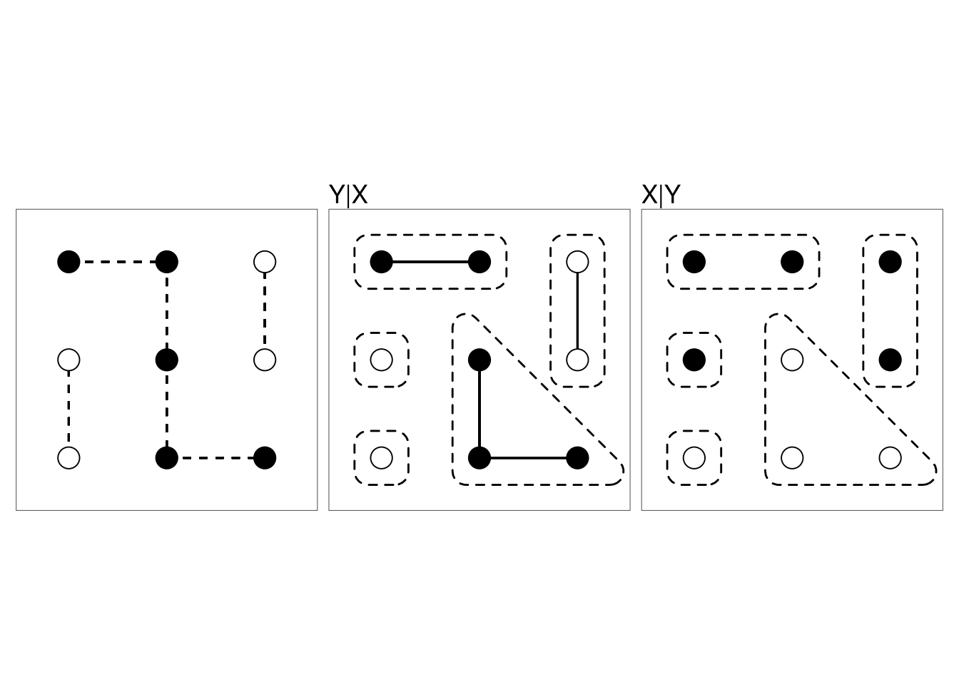
Taking \(Y_{ij}|X=x\) for \((i,j) \in \mathcal{N}\) to be independent and uniform on \([0,\exp\{\beta 1_{x_i=x_j}\}]\) makes the joint density

\[\begin{equation*} \pi(x,y) \propto \prod _{(i,j) \in \mathcal{N}} 1_{[0,\exp\{\beta 1_{x_i=x_j}\}]}(y_{ij}) \end{equation*}\]

• The conditional distribution of \(X\) given \(Y=y\) is uniform on the possible configurations.

• If \(y_{ij} > 1\) then \(x_i = x_j\); otherwise there are no further constraints.

• The nodes can be divided into patches that are constrained to be the same color.

The colors of the patches are independent and uniform on the available colors.

The algorithm that alternates generating \(Y|X\) and \(X|Y\) was introduced by Swendsen and Wang (1987).

For models without an external field this approach mixes much more rapidly than single-site updating.

Nott and Green (2004) propose a Bayesian variable selection algorithm based on the Swendsen-Wang approach.

10.12.6 Hamiltonian Monte Carlo

Hamiltonian Monte Carlo (HMC) is an auxiliary variable method for producing a Markov chain with invariant distribution \(f(\theta)\).

HMC is also known ad Hybrid Monte Carlo.

HMC requires that \(f(\theta)\) be differentiable and that the gradient of \(\log f(\theta)\) be computable.

A motivation for the method:

• View \(\theta\) as the position of an object on a surface, with potential energy \(-\log f(\theta)\).

• Add a random momentum vector \(r\), with kinetic energy \(\frac{1}{2} r \cdot r\).

• Compute where the object will be after time \(T\) by solving the differential equation of Hamiltonian dynamics.

• The numerical solution uses a discrete approximation with \(L\) steps of size \(\epsilon\), with \(T = \epsilon L\).

The random momentum values are sampled as independent standard normals.

The algorithm produces a Markov chain with invariant density

\[\begin{equation*} h(\theta, r) \propto f(\theta) \exp\left\{-\frac{1}{2} r \cdot r\right\}. \end{equation*}\]

If the differential equation is solved exactly then the \(\theta,r\) pair moves along contours of the energy surface \(-\log h(\theta, r)\).

With discretization this is not exactly true, and Metropolis Hasting step is used to correct for discretization errors.

With a good choice of \(T = \epsilon L\) the algorithm can take very large steps and mix much better than a random walk Metropolis algorithm or simple Gibbs sampler.

\(\epsilon\) has to be chosen to be large enough to move a reasonable distance but small enough to keep the acceptance probability from becoming too small.

The basic algorithm:

       Given \(\theta^0, \epsilon, L, \mathcal{L}, M\)
       for \(m = 1\) to \(M\)
           Sample \(r \sim \text{N}(0, I)\)
           Set \(\tilde{\theta}, \tilde{r} \gets \text{Leapfrog}(\theta^{m-1}, r, \epsilon, L)\)
           With probability \(\alpha = \min\left\{1, \frac{\exp\{\mathcal{L}(\tilde{\theta}) - \frac{1}{2}\tilde{r} \cdot \tilde{r}\}} {\exp\{\mathcal{L}(\theta^{m-1}) - \frac{1}{2} r \cdot r\}}\right\}\)
           set \(\theta^m \gets \tilde{\theta}\)
           Otherwise, set \(\theta^m \gets \theta^{m-1}\)
       end for

       function Leapfrog(\(\theta, r, \epsilon, L\))
           for {\(i = 1\) to \(L\)}
               Set \(r \gets r + (\epsilon / 2) \nabla_\theta \mathcal{L}(\theta)\) \(\qquad\qquad\qquad\triangleleft\) half step for \(r\)
               Set \(\theta \gets \theta + \epsilon r\) \(\qquad\qquad\qquad\qquad\qquad\triangleleft\) full step for \(\theta\)
               Set \(r \gets r + (\epsilon / 2) \nabla_\theta \mathcal{L}(\theta)\) \(\qquad\qquad\qquad\triangleleft\) another half step for \(r\)
           end for
           return \(\theta, -r\)
       end function

The Leapfrog step produces a deterministic proposal \((\tilde{\theta},\tilde{r}) = \text{Leapfrog}(\theta, r)\).

It is reversible: \((\theta,r) = \text{Leapfrog}(\tilde{\theta}, \tilde{r})\)

It is also satisfies \(|\det \nabla_{\theta,r}\text{Leapfrog}(\theta, r)| = 1\).

Without this property a Jacobian correction would be needed in the acceptance probability.

Scaling of the distribution of \(\theta\) will affect the sampler’s performance; it is useful to scale so the variation in the \(r_i\) is comparable to the variation in the \(\theta_i\).

Since \(L\) gradients are needed for each step the algorithm can be very expensive.

Pilot runs are usually used to tune \(\epsilon\) and \(L\).

It is also possible to choose values of \(\epsilon\) and \(L\) random, independently of \(\theta\) and \(r\), before each Leapfrog step

The No-U-Turn Sampler (NUTS) provides an approach to automatically tuning \(\epsilon\) and \(L\).

NUTS is the basis of the Stan framework for automate posterior sampling.

References:

Duane S, Kennedy AD, Pendleton BJ, Roweth D (1987). “Hybrid Monte Carlo.” Physics Letters, B(195), 216-222.

Neal R (2011). “MCMC for Using Hamiltonian Dynamics.” In S Brooks, A Gelman, G Jones, M Xiao-Li (eds.), Handbook of Markov Chain Monte Carlo, p. 113-162. Chapman & Hall, Boca Raton, FL.

Hoffman M, Gelman A (2012). “The No-U-Turn Sampler: Adaptively Setting Path Lengths in Hamiltonian Monte Carlo.” Journal of Machine Learning Research, 1-30.

Stan project home page.

A simple R implementation is available on line

10.12.7 Pseudo-Marginal Metropolis-Hastings MCMC

The Metropolis-Hastings method using a proposal density \(q(x, x')\) for sampling from a target proportional to \(f\) uses the acceptance ratio

\[\begin{equation*} A(x, x') = \frac{f(x') q(x', x)}{f(x)q(x, x')}. \end{equation*}\]

Sometimes the target \(f\) is expensive or impossible to compute, but a non-negative unbiased estimate is available.

Suppose, after generating a proposal \(x'\), such an estimate \(y'\) of \(f(x')\) is produced and used in the acceptance ratio

\[\begin{equation*} \hat{A}(x, x') = \frac{y' q(x', x)}{y q(x, x')}. \end{equation*}\]

The previous estimate \(y\) for \(f(x)\) has to be retained and used.

This produces a joint chain in in \(x, y\).

The marginal invariant distribution of the \(x\) component has density proportional to \(f(x)\).

To see this, denote the density of the estimate \(y\) given \(x\) as \(h(y|x)\) and write

\[\begin{equation*} \hat{A}(x, x') = \frac{y' h(y'|x')}{y h(y|x)} \frac{q(x', x)h(y | x)}{q(x, x')h(y' | x')}. \end{equation*}\]

This is the acceptance ratio for a Metropolis-Hastings chain with target density \(y h(y|x)\). Since \(y\) is unbiased, the marginal density of \(x\) is

\[\begin{equation*} \int y h(y|x) dy = f(x). \end{equation*}\]

This is known as the pseudo-marginal method introduced by Andrieu and Roberts (2009) extending earlier work of Beaumont (2003).

A number of extensions and generalizations are also available.

10.12.7.1 Doubly-Intractable Posterior Distributions

For some problems a likelihood for data \(y\) is of the form

\[\begin{equation*} p(y|\theta) = \frac{g(y, \theta)}{Z(\theta)} \end{equation*}\]

where \(g(y,\theta)\) is available but \(Z(\theta)\) is expensive or impossible to evaluate.

The posterior distribution is then

\[\begin{equation*} p(\theta|y) \propto \frac{g(y, \theta) p(\theta)}{Z(\theta)}, \end{equation*}\]

but is again not computable because of the likelihood normalizing constant \(Z(\theta)\).

For a fixed value \(\hat{\theta}\) of \(\theta\) it is useful to write the posterior density as

\[\begin{equation*} p(\theta|y) \propto g(y, \theta) p(\theta)\frac{Z(\hat{\theta})}{Z(\theta)}, \end{equation*}\]

Suppose it is possible for a given \(\theta\) to simulate a draw \(y^*\) from \(p(y|\theta)\).

Then an unbiased importance-sampling estimate of \(p(\theta|y)\) is

\[\begin{equation*} \hat{p}(\theta|y) = g(y, \theta) p(\theta)\frac{g(y^*, \hat{\theta})}{g(y^*, \theta)} \end{equation*}\]

since

\[\begin{equation*} E\left[\frac{g(y^*, \hat{\theta})}{g(y^*, \theta)}\right] = \int \frac{g(y^*, \hat{\theta})}{g(y^*, \theta)} p(y^*|\theta) dy^* = \frac{1}{Z(\theta)} \int g(y^*, \hat{\theta}) dy^* = \frac{Z(\hat{\theta})}{Z(\theta)}. \end{equation*}\]

Generating multiple \(y^*\) samples is also possible.

Reducing the variance of the estimate generally reduces rejection rates and improves mixing of the sampler.

10.12.8 Heating and Reweighting

Let \(f(x)\) have finite integral and let \(f_T(x) = f(x)^{1/T}\).

If \(f_T\) has finite integral then we can run a Markov Chain with invariant distribution \(f_T\).

Increasing \(T\) flattens the target density and may lead to a faster mixing chain—this is called heating.

Decreasing \(T\) leads to a more peaked \(f_T\) concentrated more around the global maximum of \(f\).

Careful choice of a cooling schedule \(T_n \to 0\) can produce an inhomogeneous chain that converges to the global maximum. This is called simulated annealing.

Using a fixed \(T > 1\) can produce a faster mixing chain than \(T=1\).

More generally, using a similar but more dispersed, or more easily sampled, density \(g\) may produce a faster mixing chain.

If \(X_1, X_2, \dots\) is a Markov chain with invariant density \(g\), then, under reasonable conditions,

\[\begin{equation*} \frac{\sum W_i h(X_i)}{\sum W_i} \to \frac{\int h(x) f(x) dx}{\int f(x) dx} \end{equation*}\]

where \(W_i = f(X_i)/g(X_i)\).

This approach can also be used for sensitivity analysis:

• Sample from the primary distribution of interest \(g\).

• Examine how results change for various perturbations \(f\) using the original sample from \(g\) and reweighting to \(f\).

• Reusing the sample is a form of common variate use.

Instead of keeping weights one can resample with probabilities proportional to the weights.

10.12.9 Switching and Parallel Chains

Suppose \(f_1,\dots,f_k\) are unnormalized densities, \(a_1,\dots,a_k\) are positive numbers, and \(p_{ij}\) are transition probabilities on \(\{1,\dots,k\}\).

A sampler on \((X,I)\) can be run as:

• when \(I = i\), run a sampler with invariant distribution \(f_i\) for \(K\) steps.

• Then choose an index \(J \in \{1,\dots,k\}\) with probabilities \(p_{i1},\dots,p_{ik}\).

• With probability \[\begin{equation*} \min\left\{\frac{p_{Ji} a_J f_J(X)}{p_{iJ} a_i f_i(X)}, 1\right\} \end{equation*}\] accept the proposal and set \(I = J\); otherwise keep \(I = i\)

The resulting chain has an invariant distribution with \(f(x|i) \propto f_i\).

Usually one distribution, say \(f_1\), is the primary target distribution and the others are successively “hotter” alternatives.

The hottest distribution may allow independent sampling.

This approach is called simulated tempering.

Care is needed in choosing \(a_i\) and \(p_{ij}\) to ensure the chain does not get stuck

A variant runs \(k\) chains in parallel and periodically proposes a permutation of states, which is accepted with an appropriate probability. This is called parallel tempering.

Parallel tempering does not require constants \(a_i\); the joint distribution of the chains has density proportional to \(f_1(x_1) \cdots f_k(x_k)\).

Some references:

Geyer, C. (1991) “Markov chain Monte Carlo maximum likelihood,” Computing Science and Statsitics: The 23sr Symposium on the Interface, Interface Foundation, 156–153.

Geyer, C. and Thompson, E (1995) “Annealing Markov chain Monte Carlo with applications to ancestral inference,” JASA, 909–920.

Marinari, E. and Parisi, G. (1992) “Simulated tempering: a new Monte Carlo scheme,” Europhysics letters, 451–458.

Sample code is available here

10.13 Regeneration and MCMC

A process \(X_1, X_2, \dots\) is regenerative if there exists a sequence of random variables \(T_1 \le T_2 \le T_3 \dots\) such that

• The \(T_i\) form a (possibly delayed) renewal process.

• The tour lengths and tours \[\begin{equation*} (T_{i+1}-T_i, X_{T_i+1}, X_{T_i+2}, \dots, X_{T_{i+1}}) \end{equation*}\] are independent and identically distributed.

Suppose \(X_n\) is regenerative with stationary distribution \(\pi\). Let \(T_0 = 0\), \[\begin{align*} N_i &= T_i - T_{i - 1}\\ Y_i &= \sum_{j=T_{i-1}+1}^{T_i} h(X_j) \end{align*}\]

If \(E[|Y_i|] < \infty\) and \(E[N_i] < \infty\) then

\[\begin{equation*} \widehat{\theta}_n = \frac{\sum_{i=1}^n Y_i}{\sum_{i=1}^n N_i} = \frac{\overline{Y}}{\overline{N}} \to \theta = E_\pi[h(X)] \end{equation*}\]

If \(E[Y_i^2] < \infty\) and \(E[N_i^2]<\infty\) then

\[\begin{equation*} \sqrt{n}(\widehat{\theta}_n-\theta) \to \text{N}(0,\tau) \end{equation*}\]

and \(\tau\) can be estimated by the variance estimation formula for a ratio estimator:

\[\begin{equation*} \widehat{\tau} = \frac{\frac{1}{n}\sum(Y_i-\widehat{\theta}_nN_i)^2}{\overline{N}^2} \end{equation*}\]

For a regenerative process we can simulate tours independently and in any order.

An irreducible discrete state space Markov chain is regenerative with the \(T_i\) corresponding to the hitting times of any chosen state.

Irreducible general state space chains are also regenerative.

Finding regeneration times can be hard and may involve using auxiliary variables.

If we have an approximate envelope \(h\) available, then

• we and can use Metropolized rejection sampling for a target distribution \(f\);

• every time we get \(f(X_i) \le h(X_i)\) then the next proposal will be accepted;

• so every step with \(f(X_i) \le h(X_i)\) is a regeneration time.

Periodically using a Metropolized rejection step is the simplest way to introduce regeneration in MCMC.

How well it works depends on the quality of the envelope and the other sampler it is used in conjunction with.

Other methods are available for identifying regeneration points.

Regenerative analysis does not make a sampler better: poorly mixing samplers have tour length distributions with long tails.

Sample code is available here

10.14 Transdimensional MCMC

A number of problems have parameter spaces that are unions of spaces of different dimensions:

• model selection problems;
• finite mixture models with unknown number of components;
• model-based clustering;
• partitioned regression models;
• spline models with unknown number of knots.

For each of these the parameter space can be viewed as taking the form

\[\begin{equation*} \Theta = \bigcup_{k \in \mathcal{K}} \left(\Theta_k \times \{k\}\right) \end{equation*}\]

A Bayesian formulation usually involves specifying

• a prior on \(k\);
• a conditional prior, given \(k\), on the parameters in \(\Theta_k\).

An MCMC approach needs a way of moving between models.

Several approaches are available:

• integrating out \(\theta_k\) (sometimes viable);
• reversible jump sampler;
• birth and death sampler;
• other special purpose samplers.

A useful review paper by Sisson appeared in JASA, September 2005.

10.14.1 Reversible Jump MCMC

In Bayesian model selection problems we have

• a set of \(M\) models with parameter spaces \(\Theta_1,\dots,\Theta_M\);
• a set of likelihoods \(f_i(x|\theta_i)\) with \(\theta_i \in \Theta_i\);
• conditional prior distributions given the model \(\pi(\theta_i|i)\);
• prior probabilities \(\pi(i)\) on the models.

The posterior probabilities of the models are proportional to

\[\begin{equation*} \pi(i) \int_{\Theta_i} f_i(x|\theta_i)\pi(\theta_i|i) d\theta_i \end{equation*}\]

The odds of model \(i\) to model \(j\) can be written as

\[\begin{equation*} \frac{\int_{\Theta_i} f_i(x|\theta_i)\pi(\theta_i|i) d\theta_i} {\int_{\Theta_j} f_j(x|\theta_j)\pi(\theta_j|j) d\theta_j} \frac{\pi(i)}{\pi(j)} = B_{ij}(x)\frac{\pi(i)}{\pi(j)} \end{equation*}\]

\(B_{ij}(x)\) is called the Bayes factor for model \(i\) against model \(j\).

One computational option is to run separate samplers for each model and estimate the normalizing constants.

Another option is to run a single sampler that moves both within and between models.

To move between models we need a proposal distribution \(Q_{ij}(u,dv)\) for proposing a value \(v\) in model \(j\) when currently at \(u\) in model \(i\). The proposal is accepted with probability

\[\begin{equation*} \alpha_{ij}(u,v) = \min\left\{ \frac{\pi_j(dv|x) Q_{ji}(v,du)}{\pi_i(du|x) Q_{ij}(u,dv)}, 1 \right\} = \min\left\{r_{ij}(u, v), 1\right\} \end{equation*}\]

where \(\pi_k(d\psi|x) = \pi(k) f_k(x|\psi)\pi(\psi|k) d\psi\).

With care the proposal for going from a larger model to a smaller one can be chosen to be deterministic.

This is the reversible jump sampler of Green (1995).

10.14.2 A Simple Example: Normal Means

Suppose \(X_1, X_2\) are independent.

• Model 1: \(X_1, X_2 \sim \text{N}(\mu, 1)\), \(\mu \sim N(0,b^2)\).
• Model 2: \(X_1 \sim \text{N}(\mu_1,1)\), \(X_2 \sim \text{N}(\mu_2,1)\), \(\mu_i \sim \text{N}(0, b^2)\) and independent.

The two models are assumed equally likely a priori.

The jump proposals:

• To move from 1 to 2: Generate \(\mu_1\sim \text{N}(\mu,1)\) and set \(\mu_2=2\mu-\mu_1\).
• To move from 2 to 1 set \(\mu = (\mu_1+\mu_2)/2\).

Let \(\varphi(z)\) be the standard normal density, and let

\[\begin{align*} r_{12}(\mu,\mu_1,\mu_2) &= \frac{\frac{1}{2}\varphi(x_1-\mu_1)\varphi(x_2-\mu_2) b^{-1}\varphi(\mu_1/b)d\mu_1 b^{-1}\varphi(\mu_2/b)d\mu_2} {\frac{1}{2}\varphi(x_1-\mu)\varphi(x_2-\mu)b^{-1}\varphi(\mu/b)d\mu \varphi(\mu_1-\mu)d\mu_1}\\ &= \frac{\varphi(x_1-\mu_1)\varphi(\mu_1/b)\varphi(x_2-\mu_2) \varphi(\mu_2/b)} {b\varphi(x_1-\mu)\varphi(x_2-\mu)\varphi(\mu/b)\varphi(\mu_1-\mu)} \frac{d\mu_2}{d\mu}\\ &= \frac{2}{b} \frac{\varphi(x_1-\mu_1)\varphi(\mu_1/b)\varphi(x_2-\mu_2) \varphi(\mu_2.b)} {\varphi(x_1-\mu)\varphi(x_2-\mu)\varphi(\mu/b)\varphi(\mu_1-\mu)} \end{align*}\]

Then

\[\begin{align*} \alpha_{12}(\mu,\mu_1,\mu_2) &= \min(r_{12}(\mu,\mu_1,\mu_2), 1)\\ \alpha_{21}(\mu_1, \mu_2, \mu) &= \min(1/r_{12}(\mu,\mu_1,\mu_2), 1) \end{align*}\]

R code to implement a within-model Gibbs step followed by a jump proposal:

rj <- function(m, N, x1=1, x2=-1, b=1) {
    lr12 <- function(m, m1, m2)
        log(2/b) - 0.5 * ((x1-m1)^2 + (m1/b)^2 + (x2-m2)^2 + (m2/b)^2) +
                   0.5 * ((x1-m)^2 + (x2-m)^2 + (m/b)^2 + (m1-m)^2)
    xbar <- (x1 + x2) / 2
    v <- matrix(nrow=N, ncol=3)
    I <- 1
    m <- m1 <- m2 <- 0
    for (i in 1:N) {
        if (I == 1) {
            m <- rnorm(1, xbar * b^2 / (1/2 + b^2) , b / sqrt(1 + 2 * b^2))
            m1 <- rnorm(1, m)
            m2 <- 2 * m - m1
            if (log(runif(1)) < lr12(m, m1, m2)) I <- 2
        }
        else {
            m1 <- rnorm(1, x1 * b^2 / (1 + b^2), b / sqrt(1 + b^2))
            m2 <- rnorm(1, x2 * b^2 / (1 + b^2), b / sqrt(1 + b^2))
            m <- (m1 + m2)/2
            if (log(runif(1)) < -lr12(m, m1, m2)) I <- 1
        }
        if (I == 1) v[i,] <- c(1, m, m)
        else v[i,] <- c(2, m1, m2)
    }
    v
}

Some example runs:

v <- rj(0, 10000, x1 = 2, x2 = -2, b = 1)
mean(ifelse(v[, 1] == 1, 1, 0))
## [1] 0.1422
v <- rj(0, 10000, x1 = 2, x2 = -2, b = 2)
mean(ifelse(v[, 1] == 1, 1, 0))
## [1] 0.0652
v <- rj(0, 10000, x1 = 2, x2 = -2, b = 20)
mean(ifelse(v[, 1] == 1, 1, 0))
## [1] 0.1998
v <- rj(0, 10000, x1 = 2, x2 = -2, b = 100)
mean(ifelse(v[, 1] == 1, 1, 0))
## [1] 0.5685
v<-rj(0, 10000, x1 = 2,x2 = -2, b = 200)
mean(ifelse(v[, 1] == 1, 1, 0))
## [1] 0.7148

Care is needed when using vague priors, especially when models of different dimensions are considered.

The code is available here.

10.14.3 Alternate Approach: Mixed Distributions

We can view this as a single model with means \(\mu_1,\mu_2\) and a prior distribution that says:

• with probability 1/2 the means are equal and the common value has a \(\text{N}(0,b^2)\) distribution;
• with probability 1/2 the means are unequal and drawn independently from a \(\text{N}(0,b^2)\) distribution.

The distribution of \(\mu_2|X_1,X_2,\mu_1\) is a mixed discrete-continuous distribution such that

\[\begin{align*} P(\mu_2 = \mu_1|x_1,x_2,\mu_1) &= \frac{\frac{1}{2}\varphi(x_2-\mu_1)}{\frac{1}{2}\varphi(x_2-\mu_1)+ \frac{1}{2}\frac{1}{\sqrt{1+b^2}}\varphi(x_2/\sqrt{1+b^2})}\\ &= \frac{\sqrt{1+b^2}\varphi(x_2-\mu_1)}{\sqrt{1+b^2}\varphi(x_2-\mu_1)+ \varphi(x_2/\sqrt{1+b^2})} \end{align*}\]

and

\[\begin{equation*} \mu_2|x_1,x_2,\mu_1,\mu_2\neq\mu_1 \sim \text{N}(x_2 b^2/(1+b^2),b^2/(1+b^2)) \end{equation*}\]

The conditional distribution of \(\mu_1|Y_1,Y_2,\mu_2\) is analogous.

The Gibbs sampler can therefore be used directly

Metropolis-Hastings methods can also be used if care is taken in defining densities.

With more parameters a similar approach can be used to sample pairs of parameters where the distribution can consist of

• a discrete component;
• a one dimensional component;
• a two dimensional component.

Transformations can again help: if we use

\[\begin{align*} \theta_1 &= \mu_1+\mu_2\\ \theta_2 &= \mu_1-\mu_2 \end{align*}\]

then

• \(\theta_1\),\(\theta_2\) are independent under both prior and posterior distributions;
• \(\theta_1\) has a continuous posterior distribution;
• \(\theta_2\) has a mixed posterior distribution with \(P(\theta_2 = 0|X) > 0\).

R code to implement this approach:

peq <- function(x, m, b) {
    d1 <- dnorm(x, m)
    d2 <- dnorm(x, 0, sqrt(1 + b^2))
    d1 / (d1 + d2)
}

genNeq <- function(x, m, b) {
    v <- b^2 / (1 + b^2)
    rnorm(1, x * v, sqrt(v))
}

genMu <- function(x, m, b) {
    if (runif(1) < peq(x, m, b))
        m
    else
        genNeq(x, m, b)
}

mx <- function(m, N, x1 = 2, x2 = -2, b = 1) {
    v <- matrix(nrow=N, ncol = 2)
    m1 <- m2 <- m
    for (i in 1:N) {
        m1 <- genMu(x1, m2, b)
        m2 <- genMu(x2, m1, b)
        v[i, ] <- c(m1, m2)
    }
    v
}

A sample run:

v <- mx(0, 10000)
mean(v[,1] == v[,2])
## [1] 0.1328
plot(v, asp = 1, xlab = expression(mu[1]), ylab = expression(mu[2]))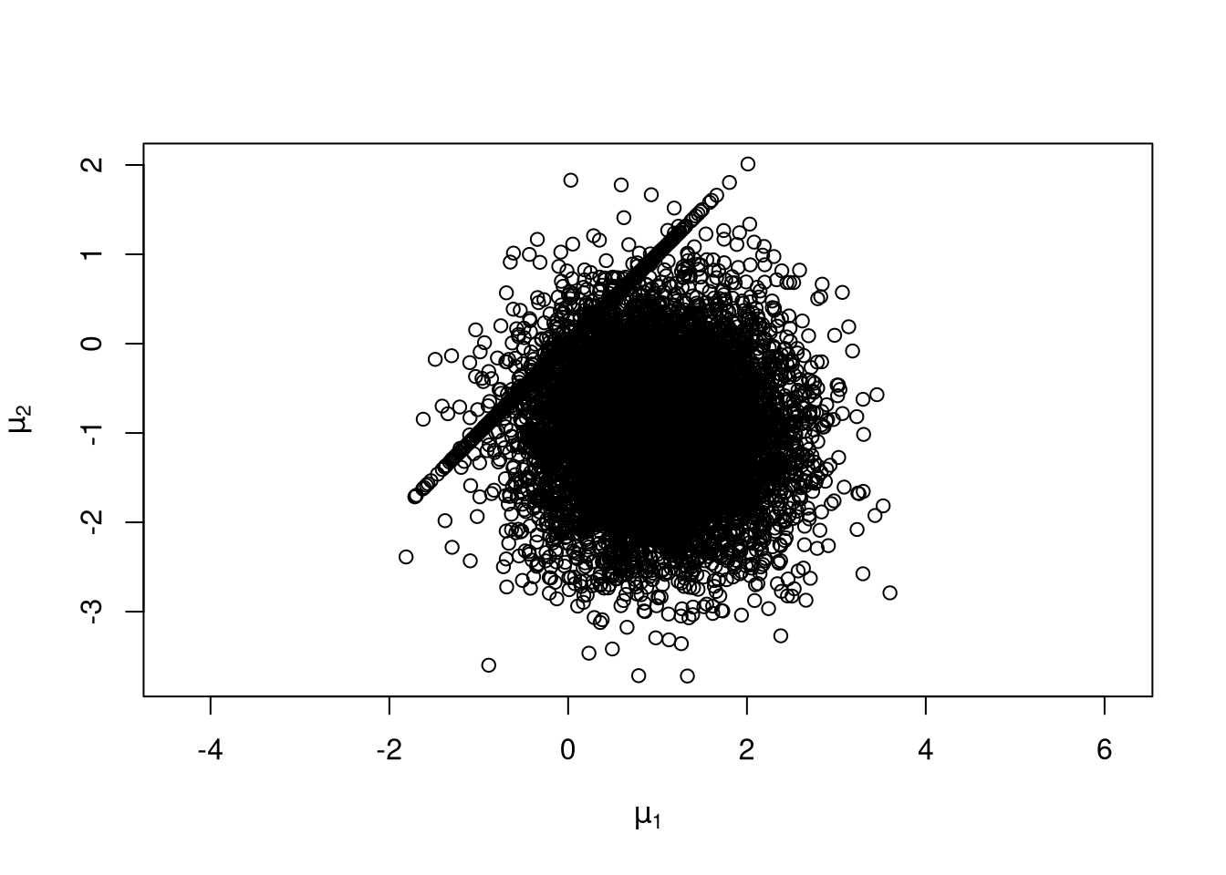

The code is available here.

10.14.4 Birth and Death MCMC

A number of models have parameters that are point processes:

• support set for finite mixture models;
• knot set for spline models.

Point process models can be sampled by a continuous time Markov process, called a spatial birth and death process.

A set of points \(y = \{y_1,\dots,y_n\}\) changes by

• births that add a point: \(y \to y \cup \{\xi\}\)
• deaths that remove a point: \(y \to y \backslash y_i\)

Births occur at a rate

\[\begin{equation*} b(y, \xi) = \beta(y) \tilde{b}(y,\xi) \end{equation*}\]

with \(\beta(y) = \int b(y, \xi) d\xi\)

The points in a set \(y = \{y_1,\dots,y_n\}\) die independently with rates \(d(y\backslash\{y_i\}, y_i)\).

The total death rate is \(\delta(y) = \sum_{i=1}^n d(y\backslash\{y_i\}, y_i)\)

Suppose we wish to simulate a point process with density \(h(y)\) with respect to an inhomogeneous Poisson process with rate \(\lambda(x)\).

A spatial birth and death process will have this point process as invariant distribution if it satisfies the detailed balance equations

\[\begin{equation*} h(y) b(y, \xi) = h(y \cup \{\xi\}) \lambda(\xi) d(y, \xi) \end{equation*}\]

Usual approach:

• pick a reasonable birth rate function;
• solve for the required death rate.

The algorithm: starting with a set of points \(y\):

1. Wait for an amount of time exponentially distributed with rate \(\beta(y)+\delta(y)\).
2. At that time, a birth occurs with probability \(\beta(y)/(\beta(y)+\delta(y))\).
3. If a birth occurs, generate the location of the new point \(\xi\) from \(\tilde{b}(y, \xi)\).
4. If a death occurs, choose the point to die with probabilities proportional to \(d(y\backslash\{y_i\},y_i)\).

The idea is due to Ripley (1977) and Preston (1977).

Stephens (2001) introduced a variation for Bayesian inference for finite mixture models.

Continuous time data for pure jump processes can be represented as the sequence of states and their waiting times.

Sample path averages are time-weighted averages.

An alternative is to sample at a discrete grid of time points.

Some notes:

• There are no rejections. Instead, some points die very quickly.
• It may be useful to add move steps that pick one point to possibly move based on, say, a Metropolis-Hastings proposal.

10.14.5 Example: Normal Mixture Models

A normal mixture model assumes that \(X_1,\dots,X_n\) are independent draws from the density

\[\begin{equation*} f(x|K, \mu, \sigma, p) = \sum_{i=1}^K p_i \frac{1}{\sigma_i}\varphi\left(\frac{x - \mu_i}{\sigma_i}\right) \end{equation*}\]

with \(\varphi\) the standard normal density and \(p_1 + \dots + p_K = 1\).

A possible prior distribution for \(K, p, \mu, \sigma\) can be specified as

\[\begin{align*} K &\sim \text{Poisson}(\lambda), \text{conditioned on $1 \le K \le K_{\max}$}\\ p | K &\sim \text{Dirichlet}(\alpha,\dots,\alpha)\\ \sigma_i^2|K,p &\overset{\text{ind}}{\sim} \text{IG}(a, b)\\ \mu_i|K,p,\sigma &\overset{\text{ind}}{\sim} \text{N}(m, c) \end{align*}\]

A more elaborate formulation might put priors on some of the hyperparameters.

If we add an auxilliary variable \(v\), independent of \(K,p,\sigma,\mu\), with

\[\begin{equation*} v | K, p, \sigma, \mu \sim \text{Gamma}\left(K \alpha, 1\right) \end{equation*}\]

and set \(w_i = v p_i\), then

\[\begin{equation*} w_i | K, \sigma, \mu \overset{\text{ind}}{\sim} \text{Gamma}(\alpha, 1) \end{equation*}\]

The prior distribution of \(K, w, \sigma^2, \mu\) is an inhomogeneous Poisson process on \(\mathbb{R}^3\) with rate function

\[\begin{align*} \lambda(\mu, \sigma, w) = \lambda &\times \text{Gamma density for $w$}\\ &\times \text{Inverse Gamma density for $\sigma^2$} \\ &\times \text{Normal density for $\mu|\sigma$} \end{align*}\]

and \(p_i = w_i / \sum_{j=1}^K w_j\), conditioned on \(1 \le K \le K_{\max}\).

The posterior distribution has a density

\[\begin{equation*} h(K, \mu, \sigma, w) \propto 1_{[1, K_{\max}]}(K)\prod_{j=1}^n f(x_i|K, \mu, \sigma, p) \end{equation*}\]

with respect to the Poisson process.

Code is available here.

10.15 Approximate Bayesian Computation (ABC)

All approaches to posterior sampling so far have required computing the likelihood function \(f(x|\theta)\).

For some problems this is not possible, but it is possible to simulate from \(f(\cdot|\theta)\).

A simple approach:

1. Draw \(\theta^*\) from the prior distribution.
2. Run the model to simulate \(x^*\) from \(f(x|\theta^*)\).
3. If \(x^*\) is close to the observed \(x\) then keep \(\theta^*\); otherwise, go back to step (1).

An MCMC variant of this is also used and can lead to higher acceptance rates.

Closeness might be measured as \(d(x, x^*) \le \epsilon\) for some distance \(d\) and tolerance \(\epsilon\).

• It the tolerance is small enough the distribution of the accepted \(\theta^*\) values should be close to the posterior distribution \(f(\theta|x)\).

• If the tolerance is too small the acceptance probability will be too low.

• This problem increases very quickly with the dimension of \(x\).

If a low dimensional sufficient statistic is available then the distance can be based on the sufficient statistic.

Generally sufficient statistics are not available in problems where ABC is needed.

If a modest number of statistics can be chosen that are nearly sufficient then the conditional distribution given these statistics may not be too far from the full posterior distribution.

Much recent literature has explored ways of selecting a suitable set of conditioning statistics.

Another direction of work explores the use of sequential Monte Carlo, and adaptive sequential Monte Carlo methods, in the ABC context (Sisson, Fan, and Tanaka, 2007).

The Wikipedia entry provides a good introduction and references.

10.16 Other MCMC and Related Approaches

There are many other approaches and ideas.

• Particle filters.
• Umbrella sampling.
• Dynamic reweighting.
• Adaptive MCMC (Christophe Andrieu, “Annotated Bibliography: Adaptive Monte Carlo Methods,” The ISBA Bulletin 15(1), March 2008; ).
• Special issue on adaptive Monte Carlo, Statistics and Computing, December 2008.
• Sequential Importance Sampling

Several book length treatments are available:

• Gamerman and Lopes (2006)
• Robert and Casella (2004)
• Chen, Shao, and Ibrahim (2000)
• Liu (2001)
• Brooks, Gelman, Jones, and Meng (2011)

among a number of others.

10.17 Perfect Sampling and Coupling From The Past

Suppose \(\pi\) is a distribution on \(E = \{1,\dots,M\}\) and \(P\) is an irreducible, aperiodic transition matrix with invariant distribution \(\pi\).

Let \(\phi(u,i)\) be the inverse CDF of \(P(i, \cdot)\), so if \(U\sim\text{U}[0,1]\) then \(\phi(U,i)\) has distribution \(P(i, \cdot)\).

Suppose \(U_1,U_2,\dots\) are independent \(\text{U}[0,1]\) and suppose

\[\begin{equation*} X_{i+1} = \phi(U_i, X_i) \end{equation*}\]

for \(i = -1, -2, \dots\).

For this chain started in the infinite past \(X_0 \sim \pi\).

Can we figure out what \(X_0\) is without going infinitely far into the past?

For \(T < 0\) and \(k \in E\) define

\[\begin{align*} X_{T}^{(T,k)} &= k\\ X_{i+1}^{(T,k)} &= \phi(U_i, X_{i}^{(T,k)}) \end{align*}\]

for \(i = T, T+1, \dots, -2, -1\).

• If \(X_0^{(T,k)}\) is the same state for all initial states \(k\), say \(X_0^{(T,k)} = j \in E\), then \(X_0 = j\). The chains are said to have coupled.
• With probability one there exists a finite \(T < 0\) such that all chains starting at T will have coupled by time zero.

The coupling from the past (CFTP) algorithm:

• Start with an initial \(T\) and determine whether all chains have coupled by time zero. If so, return the common value at time zero.
• If not, double \(T\) and repeat.

The CFTP algorithm was introduced by Propp and Wilson (1996).

If \(\phi(u, i) \le \phi(u, j)\) for every \(u\) and every \(i \le j\) then it is sufficient to consider the minimal and maximal chains \(X_i^{(T,1)}\) and \(X_i^{(T,M)}\) since

\[\begin{equation*} X_i^{(T,1)} \le X_i^{(T,k)} \le X_i^{(T,M)} \end{equation*}\]

for all \(k \in E = \{1,\dots,M\}\). If the minimal and maximal chains have coupled then all chains have coupled.

This idea can be extended to partially ordered state spaces with a minimal and maximal value.

Extensions to some continuous state space problems have been developed.

CFTP samplers for a number of interesting distributions in physics applications have been found.

Progress in statistics is still limited to somewhat artificial examples.

One issue is bias: Truncating the backward search for \(T\) will change the distribution of \(X_{0}\). Variations are available to address this.

10.17.1 Example: Image reconstruction with Ising Prior

States are partially ordered by pixel with “black” \(>\) “white”.

All “white” is minimal, all “black” is maximal.

A CFTP version of the vectorized Ising model sampler:

nn <- function(m, c) {
    nr <- nrow(m)
    nc <- ncol(m)
    nn <- matrix(0, nr, nc)
    nn[1:(nr)-1,] <- nn[1:(nr)-1,] + (m[2:nr,] == c)
    nn[2:nr,] <- nn[2:nr,] + (m[1:(nr-1),] == c)
    nn[,1:(nc)-1] <- nn[,1:(nc)-1] + (m[,2:nc] == c)
    nn[,2:nc] <- nn[,2:nc] + (m[,1:(nc-1)] == c)
    nn
}

simGroupU <- function(m, l2, l1, beta, which, u) {
    pp2 <- l2 * exp(beta * nn(m, 2))
    pp1 <- l1 * exp(beta * nn(m, 1))
    pp <- pp2 / (pp2 + pp1)
    ifelse(u[which] < pp[which], 2, 1)
}


simImgU <- function(m, img, beta, p, u) {
    white <- outer(1:nrow(m), 1:ncol(m), FUN=`+`) %% 2 == 1
    black <- ! white
    if (is.null(img)) {
        l2 <- 1
        l1 <- 1
    }
    else {
        l2 <- ifelse(img == 2, p, 1 - p)
        l1 <- ifelse(img == 1, p, 1 - p)
    }
    m[white] <- simGroupU(m, l2, l1, beta, white, u)
    m[black] <- simGroupU(m, l2, l1, beta, black, u)
    m
}

isingCFTP <- function(img, N, d, beta, p) {
    u <- array(runif(d * d * N), c(d, d, N))
    repeat {
        m1 <- matrix(1, d, d)
        m2 <- matrix(2, d, d)
        for (i in 1:dim(u)[3]) {
            m1 <- simImgU(m1, img, beta, p, u[,,i])
            m2 <- simImgU(m2, img, beta, p, u[,,i])
        }
        if (identical(m1, m2)) return (m1)
        u <- array(c(array(runif(d * d * N), c(d, d, N)), u),
                   c(d, d, 2 * N))
        N <- 2 * N
    }
}

It takes about five seconds for 10 images:

img4 <- array(0,c(64,64,10))
system.time(for (i in 1:10)
                img4[,,i] <- isingCFTP(img, 10, 64, 0.9, 0.7))
##    user  system elapsed 
##   6.689   0.183   6.907

and results for the average image seem reasonable:

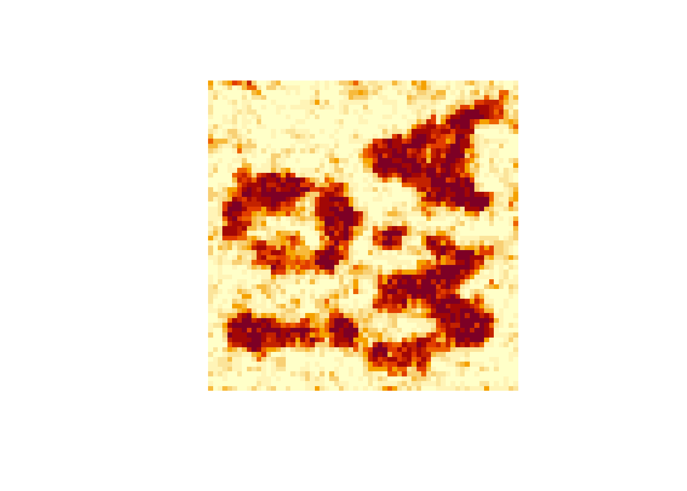
Performance deteriorates as

• dimension increases
• \(\beta\) increases

For \(\beta = 1.2\) it took about 45 seconds to generate 10 images (\(64 \times 64\))