Chapter 7 Additive Models
7.1 Basics
One approach to flexible modeling with multiple predictors is to use additive models:
\[\begin{equation*} Y = \beta_0 + f_1(x_1) + \dots + f_p(x_p) + \epsilon \end{equation*}\]
where the \(f_j\) are assumed smooth.
Variations include
some linear and some smooth terms \[Y = \beta_0 + \beta_1 x_1 + f_2(x_2) + \epsilon\]
some bivariate smooth terms \[Y = f_1(x_1) + f_{23}(x_2,x_3) + \epsilon\]
A joint model using basis functions would be of the form
\[ Y = X_0\beta + X_1\delta_1 + \dots + X_p\delta_p + \epsilon \]
with penalized objective function
\[ \|{Y - X_0\beta - \sum_{i=1}^pX_i\delta_i}\|^2 + \sum_{i=1}^p \lambda_i \delta_i^T D_i \delta_1 \]
The model can be fit using the mixed model formulation with \(p\) independent variance components.
An alternative is the backfitting algorithm.
7.2 Backfitting Algorithm
For a model
\[\begin{equation*} f(x) = \beta_0 + \sum_{j=1}^p f_j(x_j) \end{equation*}\]
with data \(y_i, x_{ij}\) and smoothers \(S_j\)
- initialize \(\widehat{\beta}_0 = \overline{y}\)
- repeat \[\begin{align*} \widehat{f}_j &\leftarrow S_j\left[\{y_i-\widehat{\beta}_0-\sum_{k \neq j} \widehat{f}_k(x_{ik})\}_1^n\right]\\ \widehat{f}_j &\leftarrow \widehat{f}_j - \frac{1}{n}\sum_{i=1}^n \widehat{f}_j(x_{ij}) \end{align*}\] until the changes in the \(\widehat{f}_j\) are below some threshold.
A more complex linear term is handled analogously.
For penalized linear smoothers with fixed smoothing parameters this can be viewed as solving the equations for the minimizer by a block Gauss-Seidel algorithm.
Different smoothers can be used on each variable.
Smoothing parameters can be adjusted during each pass or jointly.
bruto(Hastie and Tibshirani, 1990) uses a variable selection/smoothing parameter selection pass based on approximate GCV.gamfrom packagemgcvuses GCV.
Backfitting may allow larger models to be fit.
Backfitting can be viewed as one of several ways of fitting penalized/mixed models.
Some examples are available on line
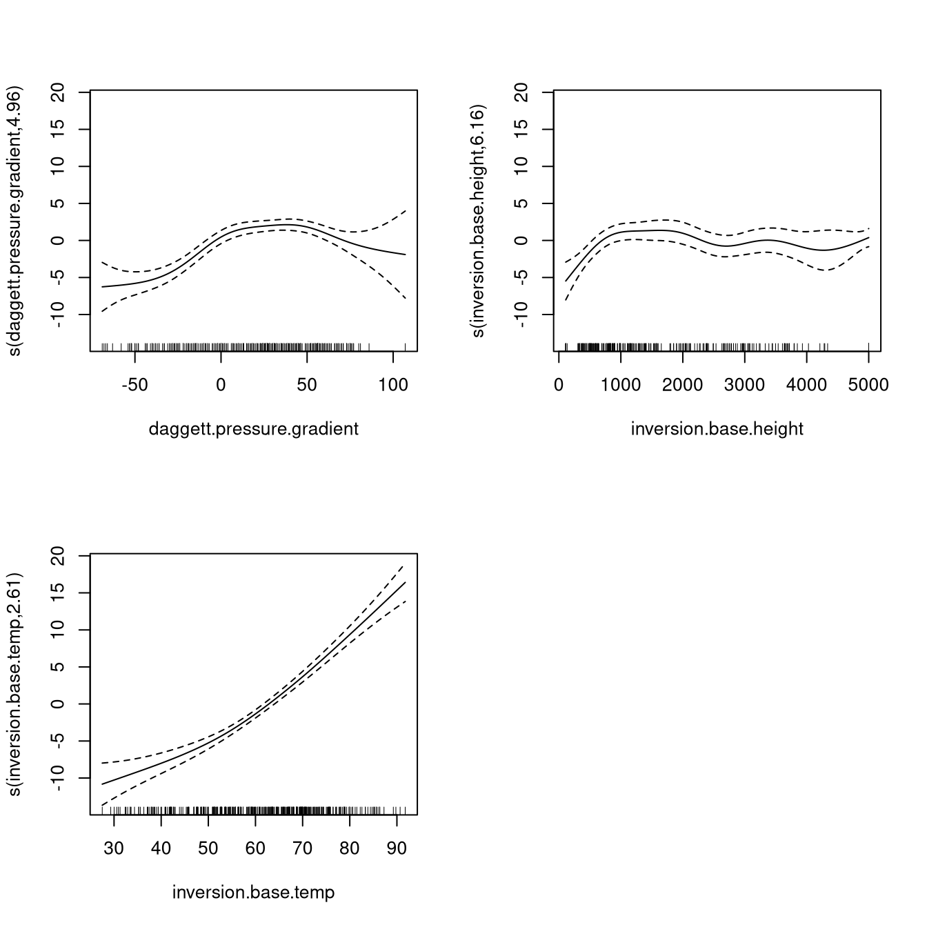
7.3 Example: Ozone Levels
Data set relates ozone levels to pressure gradient, temperature, and height of inversion.
A gam fit is produced by
library(mgcv)
data(calif.air.poll, package = "SemiPar")
fit <- gam(ozone.level ~
               s(daggett.pressure.gradient)
           + s(inversion.base.height)
           + s(inversion.base.temp),
           data = calif.air.poll)
The default plot method produces
7.4 Mixed Additive Models
Mixed additive models can be written as
\[\begin{equation*} Y = X_0 \beta + Z U + X_1 \delta_1 + \dots + X_p\delta_p + \epsilon \end{equation*}\]
where \(U\) is a “traditional” random effects term with
\[\begin{equation*} U \sim N(0,\Sigma(\theta)) \end{equation*}\]
for some parameter \(\theta\) and the terms \(X_1 \delta_1 + \dots + X_p\delta_p\) represent smooth additive terms.
In principle these can be fit with ordinary penalized least squares or mixed models software.
7.5 Example: Sitka Pines Experiment
An experiment on sitka pines measured size over time for 79 trees grown in an ozone-rich environment and a control environment.
Measurements were taken at 13 time points.
data(sitka, package = "SemiPar")
library(lattice)
sitka$ozone.char <-
    ifelse(sitka$ozone, "ozone", "control")
xyplot(log.size ~ days|ozone.char,
       groups = id.num,
       type = "b",
       data = sitka)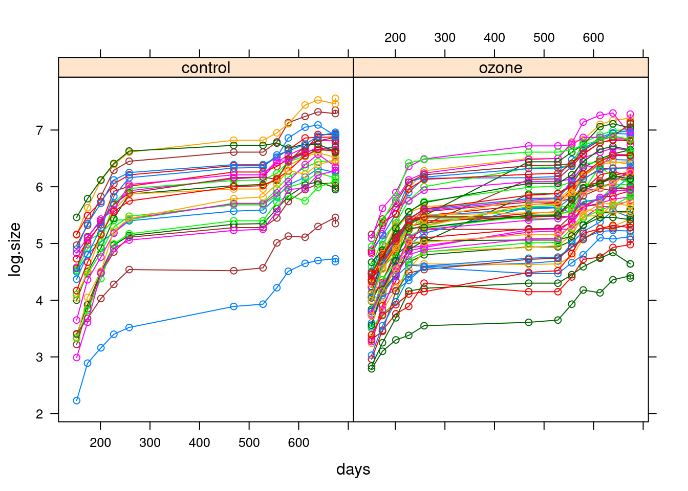
The plot suggests a model with
a smooth term for time
a mean shift for ozone
a random intercept for trees
perhaps also a random slope for trees
The random intercept model can be fit with spm using (not
working at present)
library(SemiPar)
attach(sitka)
fit <- spm(log.size ~ ozone + f(days),
           random= ~ 1, group = id.num)
and by gamm with
trees <- as.factor(sitka$id.num)
fit <- gamm(log.size ~ ozone + s(days),
            random = list(trees = ~ 1), data = sitka)
spm cannot fit a more complex random effects structure at
this point.
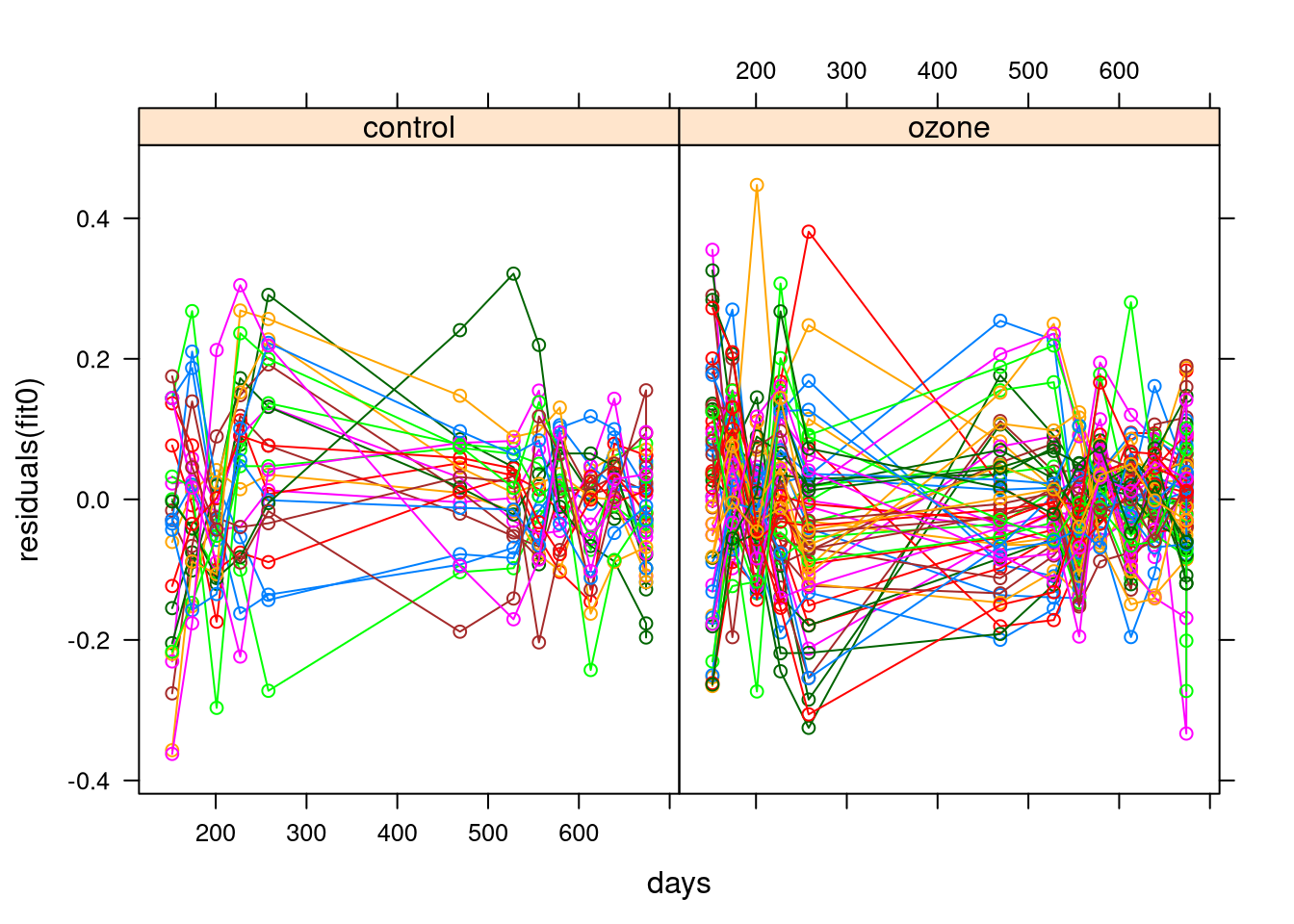
Using gamm we can fit random slope and intercept with
fit <- gamm(log.size ~ ozone + s(days),
            random = list(trees = ~ 1 + days), data = sitka)
Residuals don’t show any further obvious pattern.
Autocorrelated errors over time might be worth considering.
7.6 Generalized Additive Models
Standard generalized linear models include \[\begin{equation*} y_i \sim \text{Bernoulli}\left(\frac{\exp\{(X\beta)_i\}}{1+\exp\{(X\beta)_i\}}\right) \end{equation*}\]
and
\[\begin{equation*} y_i \sim \text{Poisson}\left(\exp\{(X\beta)_i\}\right) \end{equation*}\]
Maximum likelihood estimates can be computed by iteratively reweighted least squares (IRWLS)
Penalized maximum likelihood estimates maximize
\[\begin{equation*} \text{Loglik}(y, X_0\beta+X_i\delta) - \frac{1}{2}\lambda \delta^T D \delta \end{equation*}\]
This has a mixed model/Bayesian interpretation.
GLMM (genelarized linear mixed model) software can be used.
The IRWLS algorithm can be merged with backfitting.
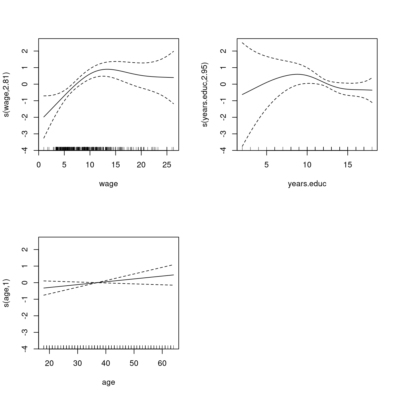
7.7 Example: Trade Union Membership
Data relating union membership and various characteristics are available.
A Bernoulli generalized additive model relates the probability of union membership to the available predictor variables.
One possible model is fit by
data(trade.union, package = "SemiPar")
fit <- gam(union.member ~ s(wage) + s(years.educ) + s(age)
                        + female + race + south,
           family=binomial,
           subset=wage < 40,    # remove high leverage point
           data=trade.union)
The estimated smooth terms are
Some summary information on the smooth terms:
summary(fit)
##
## Family: binomial
## Link function: logit
##
## Formula:
## union.member ~ s(wage) + s(years.educ) + s(age) + female + race +
##     south
##
## Parametric coefficients:
##             Estimate Std. Error z value Pr(>|z|)
## (Intercept)  -0.2434     0.4614  -0.527  0.59785
## female       -0.7101     0.2670  -2.660  0.00782 **
## race         -0.3939     0.1615  -2.439  0.01472 *
## south        -0.5209     0.2950  -1.765  0.07750 .
## ---
## Signif. codes:
## 0 '***' 0.001 '**' 0.01 '*' 0.05 '.' 0.1 ' ' 1
##
## Approximate significance of smooth terms:
##                 edf Ref.df Chi.sq  p-value
## s(wage)       2.814  3.520 22.420 0.000117 ***
## s(years.educ) 2.951  3.716  6.020 0.204710
## s(age)        1.000  1.000  2.279 0.131177
## ---
## Signif. codes:
## 0 '***' 0.001 '**' 0.01 '*' 0.05 '.' 0.1 ' ' 1
##
## R-sq.(adj) =  0.113   Deviance explained = 12.7%
## UBRE = -0.1362  Scale est. = 1         n = 533
7.8 Alternative Penalties
Bases for function spaces are infinite dimensional.
Some form of penalty or regularization is needed.
Penalties often have a useful Bayesian interpretation.
Most common penalties on coefficients \(\delta\)
quadratic, \(\sum \delta_i^2\) or, more generally, \(\delta^T D \delta\)
absolute value, \(L_1\), LASSO: \(\sum |\delta_i|\)
7.8.1 Ridge Regression
Ridge regression uses the \(L_2\) penalty \(\lambda \sum \delta_i^2\).
Using a quadratic penalty \(\delta^T D \delta\) with strictly positive definite \(D\) is sometimes called generalized ridge regression.
The minimizer of \(\|{Y - X\delta}\|^2 + \lambda \delta^T D \delta\) is
\[\begin{equation*} \widehat{\delta_\lambda} = (X^T X + \lambda D)^{-1} X^T Y \end{equation*}\]
This shrinks the OLS estimate towards zero as \(\lambda \to \infty\).
If \(X^TX = D = I\) then the ridge regression estimate is
\[\begin{equation*} \widehat{\delta_\lambda} = \frac{1}{1+\lambda}\widehat{\delta}_\text{OLS} \end{equation*}\]
7.8.2 LASSO
The LASSO (Least Absolute Shrinkage and Selection Operator) or \(L_1\)-penalized minimization problem
\[ \min_\delta\{\|{Y - X\delta}\|^2 + 2\lambda\sum |\delta_i|\} \]
does not in general have a closed form solution.
But if \(X^T X = I\) then
\[\begin{equation*} \widehat{\delta}_{i,\lambda} = \text{sign}(\widehat{\delta}_{i,\text{OLS}}) (|\widehat{\delta}_{i,\text{OLS}}| - \lambda)_{+} \end{equation*}\]
The OLS estimates are shifted towards zero and truncated at zero.
The \(L_1\) penalty approach has a Bayesian interpretation as a posterior mode for a Laplace or double exponential prior.
The variable selection property of the \(L_1\) penalty is particularly appealing when the number of regressors is large, possibly larger than the number of observations.
For least squares regression with the LASSO penalty
the solution path as \(\lambda\) varies is piece-wise linear
there are algorithms for computing the entire solution path efficiently
Common practice is to plot the coefficients \(\beta_j(\lambda)\) against the shrinkage factor \(s = \|{\beta(\lambda)}\|_1/\|{\beta(\infty)}\|_1\)
R Packages implementing general \(L_1\)-penalized regression include
lars, lasso2, and glmnet.
A paper, talk slides, and R package present a significance test for coefficients entering the model.
7.8.3 Elastic Net
The elastic net penalty is a combination of the LASSO and Ridge penalties:
\[\begin{equation*} \lambda \left[(1 - \alpha) \sum \delta_i^2 + 2 \alpha \sum |\delta_i|\right] \end{equation*}\]
Ridge regression corresponds to \(\alpha = 0\).
LASSO corresponds to \(\alpha = 1\).
\(\lambda\) and \(\alpha\) can be estimated by cross-validation.
Elastic net was introduced to address some shortcomings of LASSO, including
inability to select more than \(n\) predictors in \(p > n\) problems;
tendency to select only one of correlated predictors.
The glmnet package implements elastic net regression.
Scaling of predictors is important; by default glmnet
standardizes before fitting.
7.8.4 Non-Convex Penalties
The elastic net penalties are convex for all \(\alpha\).
This greatly simplifies the optimization to be solved.
LASSO and other elastic net fits tend to select more variables than needed.
Some non-convex penalties have the theoretical property of consistently estimating the set of covariates with non-zero coefficients under some asymptotic formulations.
Some also reduce the bias for the non-zero coefficient estimates.
Some examples are
smoothly clipped absolute deviation (SCAD);
minimax concave penalty (MCP).
MCP is of the form \(\sum \rho(\delta_i, \lambda, \gamma)\) with
\[\begin{equation*} \rho(x, \lambda, \gamma) = \begin{cases} \lambda |x| - \frac{x^2}{2\gamma} & \text{if $|x| \le \gamma\lambda$}\\ \frac{1}{2}\gamma\lambda^2 & \text{otherwise} \end{cases} \end{equation*}\]
for \(\gamma > 1\).
This behaves like \(\lambda |x|\) for small \(|x|\) and smoothly transitions to a constant for large \(|x|\). SCAD is similar in shape.
Jian Huang and Patrick Breheny have worked extensively on these.
7.9 Alternative Bases
Many other bases are used, including
polynomials
trigonometric polynomials (Fourier basis)
wavelet bases
Different bases are more suitable for modeling different functions
General idea: choose a basis in which the target can be approximated well with a small number of basis elements.
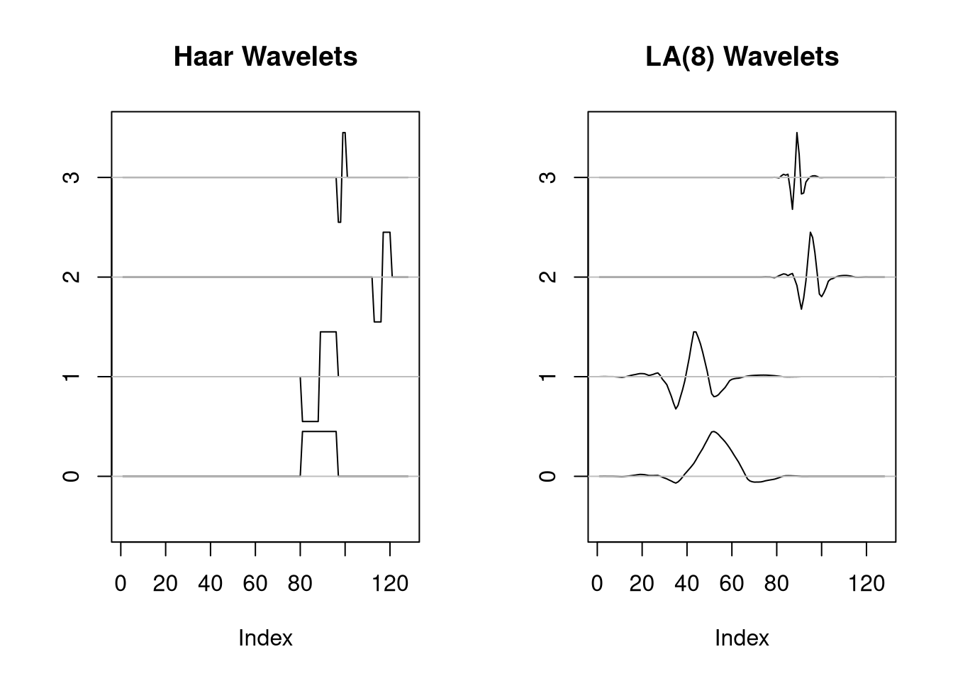
7.9.1 Wavelets
Wavelet smoothing often assumes observations at \(N=2^J\) equally spaced points and uses an orthonormal basis of \(N\) vectors organized in \(J\) levels.
Some wavelet bases:
A common approach for wavelet smoothing is to use \(L_1\) shrinkage with
\[\begin{equation*} \lambda = \widehat{\sigma} \sqrt{2\log N} \end{equation*}\]
A variant is to use different levels of smoothing at each level of detail.
\(\widehat{\sigma}\) is usually estimated by assuming the highest frequency level is pure noise.
Several R packages are available for wavelet modeling, including
waveslim, rwt, wavethresh, and
wavelets
Matlab has very good wavelet toolboxes.
S-Plus also used to have a good wavelet library.
7.10 Other Approaches
MARS, multiple adaptive regression splines. Available in the
mda package.
polymars in package polyspline.
Smoothing spline ANOVA.
Projection pursuit regression.
Single and multiple index models.
Neural networks.
Tree models.