Chapter 9 Simulation

9.1 Computer Simulation

Computer simulations are experiments performed on the computer using computer-generated random numbers.

Simulation is used to

• study the behavior of complex systems such as

  • biological systems
  • ecosystems
  • engineering systems
  • computer networks

• compute values of otherwise intractable quantities such as integrals

• maximize or minimize the value of a complicated function

• study the behavior of statistical procedures

• implement novel methods of statistical inference

Simulations need

• uniform random numbers

• non-uniform random numbers

• random vectors, stochastic processes, etc.

• techniques to design good simulations

• methods to analyze simulation results

9.2 Uniform Random Numbers

The most basic distribution is the uniform distribution on \([0,1]\)

Ideally we would like to be able to obtain a sequence of independent draws from the uniform distribution on \([0,1]\).

Since we can only use finitely many digits, we can also work with

• A sequence of independent discrete uniform random numbers on \(\{0, 1, \dots, M-1\}\) or \(\{1, 2, \dots, M\}\) for some large \(M\).

• A sequence of independent random bits with equal probability for 0 and 1.

Some methods are based on physical processes such as:

• Nuclear decay.

• Atmospheric noise; the R package random provides an interface.

• Air turbulence over disk drives or thermal noise in a semiconductor (Toshiba Random Master PCI device)

• Event timings in a computer (Linux /dev/random).

9.2.1 Using /dev/random from R

devRand <- file("/dev/random", open="rb")
U <- function()
    (as.double(readBin(devRand, "integer"))+2^31) / 2^32
x <-numeric(1000)
for (i in seq(along=x)) x[i] <- U()
hist(x)
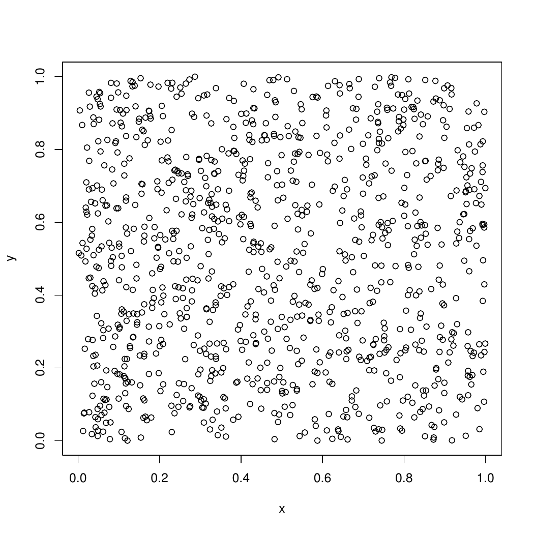
y <- numeric(1000)
for (i in seq(along=x)) y[i] <- U()
plot(x,y)
close(devRand)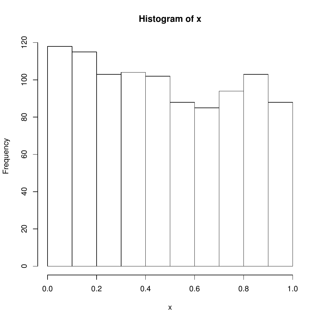

9.2.2 Issues with Physical Generators

They can be very slow.

Not reproducible except by storing all values.

The distribution is usually not exactly uniform; can be off by enough to matter.

Departures from independence may be large enough to matter.

Mechanisms, defects, are hard to study.

They can be improved by combining with other methods.

9.3 Pseudo-Random Numbers

Pseudo-random number generators produce a sequence of numbers that is

• not random;

• easily reproducible;

• “unpredictable;” “looks random”;

• behaves in many respects like a sequence of independent draws from a (discretized) uniform \([0,1]\) distribution;

• fast to produce.

Pseudo-random generators come in various qualities

• Simple generators

  • easy to implement;
  • run very fast;
  • easy to study theoretically;
  • usually have known, well understood flaws.

• More complex

  • often based on combining simpler ones;
  • somewhat slower but still very fast;
  • sometimes possible to study theoretically, often not;
  • guaranteed to have flaws; flaws may not be well understood (yet).

• Cryptographic strength

  • often much slower, more complex;
  • thought to be of higher quality;
  • may have legal complications;
  • weak generators can enable exploits; this was an issue in iOS 7.

We use mostly generators in the first two categories.

Some argue we should move to cryptographic strength ones.

9.3.1 General Properties

Most pseudo-random number generators produce a sequence of integers \(x_1, x_2, \dots\) in the range \(\{0, 1, \dots, M-1\}\) for some \(M\) using a recursion of the form

\[\begin{equation*} x_n = f(x_{n-1}, x_{n-2}, \dots, x_{n-k}) \end{equation*}\]

Values \(u_1, u_2, \dots\) are then produced by

\[\begin{equation*} u_i = g(x_{di}, x_{di-1}, \dots, x_{di - d + 1}) \end{equation*}\]

Common choices of \(M\) are

• \(M = 2^{31}\) or \(M = 2^{32}\)
• \(M = 2^{31} - 1\), a Mersenne prime
• \(M = 2\) for bit generators

The value \(k\) is the order of the generator

The set of the most recent \(k\) values is the state of the generator.

The initial state \(x_1, \dots, x_k\) is called the seed.

Since there are only finitely many possible states, eventually these generators will repeat.

The length of a cycle is called the period of a generator.

The maximal possible period is on the order of \(M^k\)

Needs change:

• As computers get faster, larger, more complex simulations are run.

• A generator with period \(2^{32}\) used to be good enough.

• A current computer can run through \(2^{32}\) pseudo-random numbers in under one minute.

• Most generators in current use have periods \(2^{64}\) or more.

• Parallel computation also raises new issues.

9.3.2 Linear Congruential Generators

A linear congruential generator is of the form

\[\begin{equation*} x_i = (a x_{i-1} +c) \mod M \end{equation*}\]

with \(0 \le x_i < M\).

• \(a\) is the multiplier
• \(c\) is the increment
• \(M\) is the modulus

A multiplicative generator is of the form

\[\begin{equation*} x_i = a x_{i-1} \mod M \end{equation*}\]

with \(0 < x_i < M\).

A linear congruential generator has full period \(M\) if and only if three conditions hold:

• \(\gcd(c,M) = 1\)
• \(a \equiv 1 \mod p\) for each prime factor \(p\) of \(M\)
• \(a \equiv 1 \mod 4\) if 4 divides \(M\)

A multiplicative generator has period at most \(M-1\). Full period is achieved if and only if \(M\) is prime and \(a\) is a primitive root modulo \(M\), i.e. \(a \neq 0\) and \(a^{(M-1)/p} \not \equiv 1 \mod M\) for each prime factor \(p\) of \(M-1\).

9.3.2.1 Examples

Lewis, Goodman, and Miller (``minimal standard’’ of Park and Miller):

\[\begin{equation*} x_i = 16807 x_{i-1} \mod (2^{31}-1) = 7^5 x_{i-1} \mod (2^{31}-1) \end{equation*}\]

Reasonable properties, period \(2^{31}-2 \approx 2.15 * 10^9\) is very short for modern computers.

RANDU:

\[\begin{equation*} x_i = 65538 x_{i-1} \mod 2^{31} \end{equation*}\]

Period is only \(2^{29}\) but that is the least of its problems:

\[\begin{equation*} u_{i+2} - 6 u_{i+1} + 9 u_{i} = \text{an integer} \end{equation*}\]

so \((u_{i}, u_{i+1}, u_{i+2})\) fall on 15 parallel planes.

Using the randu data set and the rgl package:

library(rgl)
points3d(randu)
par3d(FOV=1)  ## removes perspective distortion

With a larger number of points:

seed <- as.double(1)
RANDU <- function() {
    seed <<- ((2^16 + 3) * seed) %% (2^31)
    seed/(2^31)
}

U <- matrix(replicate(10000 * 3, RANDU()), ncol = 3, byrow = TRUE)
clear3d()
points3d(U)
par3d(FOV=1)

This generator used to be the default generator on IBM 360/370 and DEC PDP11 machines.

Some examples are available on line.

9.3.2.2 Lattice Structure

All linear congruential sequences have a lattice structure

Methods are available for computing characteristics, such as maximal distance between adjacent parallel planes

Values of \(M\) and \(a\) can be chosen to achieve good lattice structure for \(c = 0\) or \(c = 1\); other values of \(c\) are not particularly useful.

9.3.3 Shift-Register Generators

Shift-register generators take the form

\[\begin{equation*} x_i = a_1 x_{i-1} + a_2 x_{i-2} + \dots + a_p x_{i-p} \mod 2 \end{equation*}\]

for binary constants \(a_1, \dots, a_p\).

values in \([0,1]\) are often constructed as

\[\begin{equation*} u_i = \sum_{s=1}^L 2^{-s}x_{ti + s} = 0.x_{it+1}x_{it+2}\dots x_{it+L} \end{equation*}\]

for some \(t\) and \(L \le t\). \(t\) is the decimation.

The maximal possible period is \(2^p-1\) since all zeros must be excluded.

The maximal period is achieved if and only if the polynomial

\[\begin{equation*} z^p + a_1 z^{p-1} + \dots + a_{p-1} z + a_p \end{equation*}\]

is irreducible over the finite field of size 2.

Theoretical analysis is based on \(k\)-distribution: A sequence of \(M\) bit integers with period \(2^p-1\) is \(k\)-distributed if every \(k\)-tuple of integers appears \(2^{p-kM}\) times, except for the zero tuple, which appears one time fewer.

Generators are available that have high periods and good \(k\)-distribution properties.

9.3.4 Lagged Fibonacci Generators

Lagged Fibonacci generators are of the form

\[\begin{equation*} x_i = (x_{i - k} \circ x_{i - j}) \mod M \end{equation*}\]

for some binary operator \(\circ\).

Knuth recommends

\[\begin{equation*} x_i = (x_{i - 100} - x_{i-37}) \mod 2^{30} \end{equation*}\]

There are some regularities if the full sequence is used; one recommendation is to generate in batches of 1009 and use only the first 100 in each batch.

Initialization requires some care.

9.3.5 Combined Generators

Combining several generators may produce a new generator with better properties.

Combining generators can also fail miserably.

Theoretical properties are often hard to develop.

Wichmann-Hill generator:

\[\begin{align*} x_i &= 171 x_{i-1} \mod 30269\\ y_i &= 172 y_{i-1} \mod 30307\\ z_i &= 170 z_{i-1} \mod 30323 \end{align*}\]

and

\[\begin{equation*} u_i = \left(\frac{x_i}{30269} + \frac{y_i}{30307} + \frac{z_i}{30232}\right) \mod 1 \end{equation*}\]

The period is around \(10^{12}\).

This turns out to be equivalent to a multiplicative generator with modulus

\[\begin{equation*} M = 27 817 185 604 309 \end{equation*}\]

Marsaglia’s Super-Duper used in S-PLUS and others combines a linear congruential and a feedback-shift generator.

9.3.6 Other Generators

Mersenne twister;

Marsaglia multicarry;

Parallel generators:

• SPRNG.

• L’Ecuyer, Simard, Chen, and Kelton

9.3.7 Pseudo-Random Number Generators in R

R provides a number of different basic generators:

• Wichmann-Hill: Period around \(10^{12}\)

• Marsaglia-Multicarry: Period at least \(10^{18}\)

• Super-Duper: Period around \(10^{18}\) for most seeds; similar to S-PLUS

• Mersenne-Twister: Period \(2^{19937} - 1 \approx 10^{6000}\); equidistributed in 623 dimensions; current default in R.

• Knuth-TAOCP: Version from second edition of The Art of Computer Programming, Vol. 2; period around \(10^{38}\).

• Knuth-TAOCP-2002: From third edition; differs in initialization.

• L’Ecuyer-CMRG: A combined multiple-recursive generator from L’Ecuyer (1999). The period is around \(2^{191}\). This provides the basis for the multiple streams used in package parallel.

• user-supplied: Provides a mechanism for installing your own generator; used for parallel generation by

  • rsprng package interface to SPRNG
  • rlecuyer package interface to L’Ecuyer, Simard, Chen, and Kelton system
  • rstreams package, another interface to L’Ecuyer et al.

9.3.8 Testing Generators

All generators have flaws; some are known, some are not (yet).

Tests need to look for flaws that are likely to be important in realistic statistical applications.

Theoretical tests look for

• bad lattice structure
• lack of \(k\)-distribution
• other tractable properties

Statistical tests look for simple simulations where pseudo-random number streams produce results unreasonably far from known answers.

Some batteries of tests:

• DIEHARD
• DIEHARDER
• NIST Test Suite
• TestU01

9.3.9 Issues and Recommendations

Good choices of generators change with time and technology:

• Faster computers need longer periods.
• Parallel computers need different methods.

All generators are flawed

• Bad simulation results due to poor random number generators are very rare; coding errors in simulations are not.

• Testing a generator on a similar problem with known answers is a good idea (and may be useful to make results more accurate).

• Using multiple generators is a good idea; R makes this easy to do.

• Be aware that some generators can produce uniforms equal to 0 or 1 (I believe R’s will not).

• Avoid methods that are sensitive to low order bits

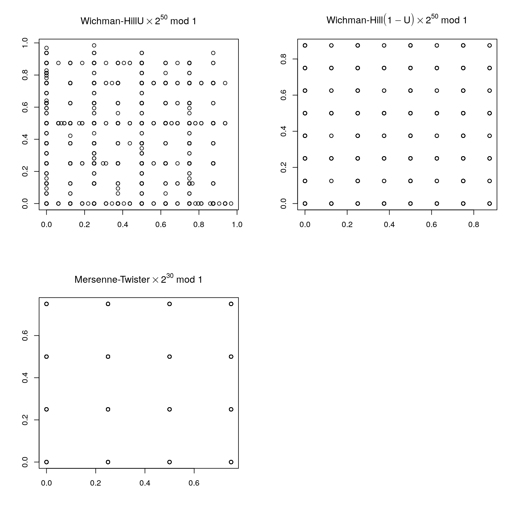
Again some examples are available on line.

9.4 Non-Uniform Random Variate Generation

Starting point: Assume we can generate a sequence of independent uniform \([0,1]\) random variables.

Develop methods that generate general random variables from uniform ones.

Considerations:

• Simplicity, correctness;

• Accuracy, numerical issues;

• Speed:

  • Setup;
  • Generation.

General approaches:

• Univariate transformations;

• Multivariate transformations;

• Mixtures;

• Accept/Reject methods.

9.4.1 Inverse CDF Method

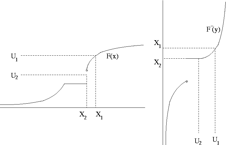
Suppose \(F\) is a cumulative distribution function (CDF). Define the inverse CDF as

\[\begin{equation*} F^{-}(u) = \min \{x: F(x) \ge u\} \end{equation*}\]

If \(U \sim \text{U}[0,1]\) then \(X = F^{-}(U)\) has CDF \(F\).

Since \(F\) is right continuous, the minimum is attained. Therefore \(F(F^{-}(u)) \ge u\) and \(F^{-}(F(x)) = \min\{y:F(y) \ge F(x)\}\). So

\[\begin{equation*} \{(u,x): F^{-}(u) \le x\} = \{(u,x): u \le F(x)\} \end{equation*}\]

and thus \(P(X \le x) = P(F^{-}(U) \le x) = P(U \le F(x)) = F(x)\).

9.4.1.1 Example: Unit Exponential Distribution

The unit exponential CDF is

\[\begin{equation*} F(x) = \begin{cases} 1-e^{-x} & \text{for $x > 0$}\\ 0 & \text{otherwise} \end{cases} \end{equation*}\]

with inverse CDF

\[\begin{equation*} F^{-}(u) = -\log(1-u) \end{equation*}\]

So \(X = -\log(1-U)\) has an exponential distribution.

Since \(1-U \sim \text{U}[0,1]\), \(-\log U\) also has a unit exponential distribution.

If the uniform generator can produce 0, then these should be rejected.

9.4.1.2 Example: Standard Cauchy Distribution

The CDF of the standard Cauchy distribution is

\[\begin{equation*} F(x) = \frac{1}{2} + \frac{1}{\pi}\arctan(x) \end{equation*}\]

with inverse CDF

\[\begin{equation*} F^{-}(u) = \tan(\pi(u-1/2)) \end{equation*}\]

So \(X = \tan(\pi(U-1/2))\) has a standard Cauchy distribution.

An alternative form is: Let \(U_1, U_2\) be independent \(\text{U}[0,1]\) random variables and set

\[\begin{equation*} X = \begin{cases} \tan(\pi(U_2/2) & \text{if $U_1 \ge 1/2$}\\ -\tan(\pi(U_2/2) & \text{if $U_1 < 1/2$}\\ \end{cases} \end{equation*}\]

• \(U_1\) produces a random sign
• \(U_2\) produces the magnitude
• This will preserve fine structure of \(U_2\) near zero, if there is any.

9.4.1.3 Example: Standard Normal Distribution

The CDF of the standard normal distribution is

\[\begin{equation*} \Phi(x) = \int_{-\infty}^x \frac{1}{\sqrt{2\pi}} e^{-z^2/2} dz \end{equation*}\]

and the inverse CDF is \(\Phi^{-1}\).

Neither \(\Phi\) nor \(\Phi^{-1}\) are available in closed form.

Excellent numerical routines are available for both.

Inversion is currently the default method for generating standard normals in R.

The inversion approach uses two uniforms to generate one higher-precision uniform via the code

    case INVERSION:
#define BIG 134217728 /* 2^27 */
        /* unif_rand() alone is not of high enough precision */
        u1 = unif_rand();
        u1 = (int)(BIG*u1) + unif_rand();
        return qnorm5(u1/BIG, 0.0, 1.0, 1, 0);

9.4.1.4 Example: Geometric Distribution

The geometric distribution with PMF \(f(x) = p(1-p)^x\) for \(x = 0, 1, \dots\), has CDF

\[\begin{equation*} F(x) = \begin{cases} 1 - (1 - p)^{\lfloor x + 1\rfloor} & \text{for $x \ge 0$}\\ 0 & \text{for $x < 0$} \end{cases} \end{equation*}\]

where \(\lfloor y \rfloor\) is the integer part of \(y\). The inverse CDF is

\[\begin{align*} F^{-}(u) &= \lceil \log(1-u)/ \log(1-p) \rceil - 1\\ &= \lfloor \log(1-u)/ \log(1-p) \rfloor & \text{except at the jumps} \end{align*}\]

for \(0 < u < 1\). So \(X = \lfloor \log(1-U)/ \log(1-p) \rfloor\) has a geometric distribution with success probability \(p\).

Other possibilities:

\[\begin{equation*} X = \lfloor \log(U)/ \log(1-p) \rfloor \end{equation*}\]

or

\[\begin{equation*} X = \lfloor -Y / \log(1-p) \rfloor \end{equation*}\]

where \(Y\) is a unit exponential random variable.

9.4.1.5 Example: Truncated Normal Distribution

Suppose \(X \sim \text{N}(\mu, 1)\) and

\[\begin{equation*} y \sim X | X > 0. \end{equation*}\]

The CDF of \(Y\) is

\[\begin{equation*} F_Y(y) = \begin{cases} \frac{P(0 < X \le y)}{P(0 < X)} & \text{for $y \ge 0$}\\ 0 & \text{for $y < 0$} \end{cases} = \begin{cases} \frac{F_X(y) - F_X(0)}{1 - F_X(0)} & \text{for $y \ge 0$}\\ 0 & \text{for $y < 0$} \end{cases}. \end{equation*}\]

The inverse CDF is

\[\begin{equation*} F_Y^{-1}(u) = F_X^{-1}(u(1-F_X(0)) + F_X(0)) = F_X^{-1}(u + (1-u)F_X(0)). \end{equation*}\]

An R function corresponding to this definition is

Q1 <- function(p, m) qnorm(p + (1 - p)* pnorm(0, m), m)

This seems to work well for positive \(\mu\) but not for negative values far from zero:

Q1(0.5, c(1, 3, 5, 10, -10))
## [1]  1.200174  3.001692  5.000000 10.000000       Inf

The reason is that pnorm(0, -10) is rounded to one.

A mathematically equivalent formulation of the inverse CDF is

\[\begin{equation*} F_Y^{-1}(u) = F_X^{-1}(1 - (1 - u)(1 - F_X(0))) \end{equation*}\]

which leads to

Q2 <- function(p, m)
    qnorm((1 - p)* pnorm(0, m, lower.tail = FALSE),
          m, lower.tail = FALSE)

and

Q2(0.5, c(1, 3, 5, 10, -10))
## [1]  1.20017369  3.00169185  5.00000036 10.00000000
## [5]  0.06841184

9.4.1.6 Issues

In principle, inversion can be used for any distribution.

Sometimes routines are available for \(F^{-}\) but are quite expensive:

system.time(rbeta(1000000, 2.5, 3.5))
##    user  system elapsed 
##   0.111   0.001   0.112
system.time(qbeta(runif(1000000), 2.5, 3.5))
##    user  system elapsed 
##   1.668   0.000   1.671

rbeta is about 20 times faster than inversion.

If \(F^{-}\) is not available but \(F\) is, then one can solve the equation \(u=F(x)\) numerically for \(x\).

Accuracy of \(F\) or \(F^{-}\) may be an issue, especially when writing code for a parametric family that is to work well over a wide parameter range.

Even when inversion is costly,

• the cost of random variate generation may be a small fraction of the total cost of a simulation;
• using inversion creates a simple relation between the variables and the underlying uniforms that may be useful.

9.4.2 Multivariate Transformations

Many distributions can be expressed as the marginal distribution of a function of several variables.

9.4.2.1 Box-Muller Method for the Standard Normal Distribution

Suppose \(X_1\) and \(X_2\) are independent standard normals. The polar coordinates \(\theta\) and \(R\) are independent,

• \(\theta\) is uniform on \([0,2\pi)\)
• \(R^2\) is \(\chi_2^2\), which is exponential with mean 2

So if \(U_1\) and \(U_2\) are independent and uniform on \([0,1]\), then

\[\begin{align*} X_1 &= \sqrt{-2\log U_1} \cos(2 \pi U_2)\\ X_2 &= \sqrt{-2\log U_1} \sin(2 \pi U_2) \end{align*}\]

are independent standard normals. This is the Box-Muller method.

9.4.2.2 Polar Method for the Standard Normal Distribution

The trigonometric functions are somewhat slow to compute. Suppose \((V_1,V_2)\) is uniform on the unit disk

\[\begin{equation*} \{(v_1,v_2): v_1^2 + v_2^2 \le 1\} \end{equation*}\]

Let \(R^2 = V_1^2 + V_2^2\) and

\[\begin{align*} X_1 &= V_1 \sqrt{-(2\log{R^2})/R^2}\\ X_2 &= V_2 \sqrt{-(2\log{R^2})/R^2} \end{align*}\]

Then \(X_1, X_2\) are independent standard normals.

This is the polar method of Marsaglia and Bray.

Generating points uniformly on the unit disk can be done using rejection sampling, or accept/reject sampling:

   repeat        generate independent \(V_1, V_2 \sim \text{U}(-1,1)\)    until \(V_1^2 + V_2^2 \le 1\)    return \((V_1, V_2)\)

This independently generates pairs \((V_1, V_2)\) uniformly on the square \((-1,1) \times (-1,1)\) until the result is inside the unit disk.

• The resulting pair is uniformly distributed on the unit disk.

• The number of pairs that need to be generated is a geometric variable with success probability \[\begin{equation*} p = \frac{\text{area of disk}}{\text{area of square}} = \frac{\pi}{4} \end{equation*}\]

  The expected number of generations needed is \(1/p = 4/\pi = 1.2732\).

• The number of generations needed is independent of the final pair.

9.4.2.3 Polar Method for the Standard Cauchy Distribution

The ratio of two standard normals has a Cauchy distribution.

Suppose two standard normals are generated by the polar method,

\[\begin{align*} X_1 &= V_1 \sqrt{-(2\log{R^2})/R^2}\\ X_2 &= V_2 \sqrt{-(2\log{R^2})/R^2} \end{align*}\]

with \(R^2 = V_1^2 + V_2^2\) and \((V_1,V_2)\) uniform on the unit disk.

Then

\[\begin{equation*} Y = \frac{X_1}{X_2} = \frac{V_1}{V_2} \end{equation*}\]

is the ratio of the two coordinates of the pair that is uniformly distributed on the unit disk.

This idea leads to a general method, the Ratio-of-Uniforms method.

9.4.2.4 Student’s t Distribution

Suppose

• \(Z\) has a standard normal distribution,
• \(Y\) has a \(\chi_\nu^2\) distribution,
• \(Z\) and \(Y\) are independent.

Then

\[\begin{equation*} X = \frac{Z}{\sqrt{Y/\nu}} \end{equation*}\]

has a \(t\) distribution with \(\nu\) degrees of freedom.

To use this representation we will need to be able to generate from a \(\chi_\nu^2\) distribution, which is a \(\text{Gamma}(\nu/2,2)\) distribution.

9.4.2.5 Beta Distribution

Suppose \(\alpha > 0\), \(\beta > 0\), and

• \(U \sim \text{Gamma}(\alpha, 1)\)
• \(V \sim \text{Gamma}(\beta, 1)\)
• \(U, V\) are independent

Then

\[\begin{equation*} X = \frac{U}{U+V} \end{equation*}\]

has a \(\text{Beta}(\alpha, \beta)\) distribution.

9.4.2.6 F Distribution

Suppose \(a > 0\), \(b > 0\), and

• \(U \sim \chi_a^2\)
• \(V \sim \chi_b^2\)
• \(U, V\) are independent

Then

\[\begin{equation*} X = \frac{U/a}{V/b} \end{equation*}\]

has an F distribution with \(a\) and \(b\) degrees of freedom.

Alternatively, if \(Y \sim \text{Beta}(a/2, b/2)\), then

\[\begin{equation*} X = \frac{b}{a}\frac{Y}{1-Y} \end{equation*}\]

has an F distribution with \(a\) and \(b\) degrees of freedom.

9.4.2.7 Non-Central t Distribution

Suppose

• \(Z \sim \text{N}(\mu, 1)\),
• \(Y \sim \chi_\nu^2\),
• \(Z\) and \(Y\) are independent.

Then

\[\begin{equation*} X = \frac{Z}{\sqrt{Y/\nu}} \end{equation*}\]

has non-central \(t\) distribution with \(\nu\) degrees of freedom and non-centrality parameter \(\mu\).

9.4.2.8 Non-Central Chi-Square, and F Distributions

Suppose

• \(Z_1, \dots, Z_k\) are independent
• \(Z_i \sim \text{N}(\mu_i,1)\)

Then

\[\begin{equation*} Y = Z_1^2 + \dots + Z_k^2 \end{equation*}\]

has a non-central chi-square distribution with \(k\) degrees of freedom and non-centrality parameter

\[\begin{equation*} \delta = \mu_1^2 + \dots + \mu_k^2 \end{equation*}\]

An alternative characterization: if \(\widetilde{Z}_1, \dots, \widetilde{Z}_k\) are independent standard normals then

\[\begin{equation*} Y = (\widetilde{Z}_1 + \sqrt{\delta})^2 + \widetilde{Z}_2^2 \dots + \widetilde{Z}_k^2 = (\widetilde{Z}_1 + \sqrt{\delta})^2 + \sum_{i=2}^k \widetilde{Z}_i^2 \end{equation*}\]

has a non-central chi-square distribution with \(k\) degrees of freedom and non-centrality parameter \(\delta\).

The non-central F is of the form

\[\begin{equation*} X = \frac{U/a}{V/b} \end{equation*}\]

where \(U\), \(V\) are independent, \(U\) is a non-central \(\chi_a^2\) and \(V\) is a central \(\chi_b^2\) random variable.

9.4.2.9 Bernoulli and Binomial Distributions

Suppose \(p \in [0,1]\), \(U \sim \text{U}[0,1]\), and

\[\begin{equation*} X = \begin{cases} 1 & \text{if $U \le p$}\\ 0 & \text{otherwise} \end{cases} \end{equation*}\]

Then \(X\) bas a \(\text{Bernoulli}(p)\) distribution.

If \(Y_1, \dots, Y_n\) are independent \(\text{Bernoulli}(p)\) random variables, then

\[\begin{equation*} X = Y_1 + \dots + Y_n \end{equation*}\]

has a \(\text{Binomial}(n,p)\) distribution.

For small \(n\) this is an effective way to generate binomials.

9.4.3 Mixtures and Conditioning

Many distributions can be expressed using a hierarchical structure:

\[\begin{align*} X|Y &\sim f_{X|Y}(x|y)\\ Y &\sim f_Y(y) \end{align*}\]

The marginal distribution of \(X\) is called a mixture distribution. We can generate \(X\) by

   Generate \(Y\) from \(f_Y(y)\).    Generate \(X|Y=y\) from \(f_{X|Y}(x|y)\).

9.4.3.1 Student’s t Distribution

Another way to think of the \(t_\nu\) distribution is:

\[\begin{align*} X|Y &\sim \text{N}(0, \nu/Y)\\ Y &\sim \chi_\nu^2 \end{align*}\]

The \(t\) distribution is a scale mixture of normals.

Other choices of the distribution of \(Y\) lead to other distributions for \(X\).

9.4.3.2 Negative Binomial Distribution

The negative binomial distribution with PMF

\[\begin{equation*} f(x) = \binom{x+r-1}{r-1}p^r(1-p)^x \end{equation*}\]

for \(x=0, 1, 2, \dots,\) can be written as a gamma mixture of Poissons: if

\[\begin{align*} X|Y &\sim \text{Poisson}(Y)\\ Y &\sim \text{Gamma}(r, (1-p)/p) \end{align*}\]

then \(X \sim \text{Negative Binomial}(r, p)\).

[The notation \(\text{Gamma}(\alpha,\beta)\) means that \(\beta\) is the scale parameter.]

This representation makes sense even when \(r\) is not an integer.

9.4.3.3 Non-Central Chi-Square

The density of the non-central \(\chi_\nu^2\) distribution with non-centrality parameter \(\delta\) is

\[\begin{equation*} f(x) = e^{-\delta/2} \sum_{i=0}^\infty \frac{(\delta/2)^i}{i!} f_{\nu+2i}(x) % I think Monahan's formula is wrong and this is right: % f(x) = exp(-lambda/2) SUM_{r=0}^infty (lambda^r / 2^r r!) pchisq(x, df + 2r) \end{equation*}\]

where \(f_k(x)\) central \(\chi^2_k\) density. This is a Poisson-weighted average of \(\chi^2\) densities, so if

\[\begin{align*} X|Y &\sim \chi_{\nu+2Y}^2\\ Y &\sim \text{Poisson}(\delta/2) \end{align*}\]

then \(X\) has a non-central \(\chi_\nu^2\) distribution with non-centrality parameter \(\delta\).

9.4.3.4 Composition Method

Suppose we want to sample from the density

\[\begin{equation*} f(x) = \begin{cases} x/2 & 0 \le x < 1\\ 1/2 & 1 \le x < 2\\ 3/2 - x/2 & 2 \le x \le 3\\ 0 & \text{otherwise} \end{cases} \end{equation*}\]

We can write \(f\) as the mixture

\[\begin{equation*} f(x) = \frac{1}{4} f_1(x) + \frac{1}{2} f_2(x) + \frac{1}{4} f_3(x) \end{equation*}\]

with

\[\begin{align*} f_1(x) &= 2x & 0 \le x < 1\\ f_2(x) &= 1 & 1 \le x < 2\\ f_3(x) &= 6-2x & 2 \le x \le 3 \end{align*}\]

and \(f_i(x) = 0\) for other values of \(x\).

Generating from the \(f_i\) is straight forward. So we can sample from \(f\) using:

   Generate \(I\) from \(\{1, 2, 3\}\) with probabilities \(1/4, 1/2, 1/4\).    Generate \(X\) from \(f_I(x)\) by inversion.

This approach can be used in conjunction with other methods.

One example: The polar method requires sampling uniformly from the unit disk. This can be done by

• encloseing the unit disk in a regular hexagon;
• using composition to sample uniformly from the hexagon until the result is in the unit disk.

9.4.3.5 Alias Method

Suppose \(f(x)\) is a probability mass function on \(\{1, 2, \dots, k\}\). Then \(f(x)\) can be written as

\[\begin{equation*} f(x) = \sum_{i=1}^k \frac{1}{k} f_i(x) \end{equation*}\]

where

\[\begin{equation*} f_i(x) = \begin{cases} q_i & x = i\\ 1-q_i & x = a_i\\ 0 & \text{otherwise} \end{cases} \end{equation*}\]

for some \(q_i \in [0,1]\) and some \(a_i \in \{1, 2, \dots, k\}\).

Once values for \(q_i\) and \(a_i\) have been found, generation is easy:

   Generate \(I\) uniform on \(\{1, \dots ,k\}\)    Generate \(U\) uniform on \([0,1]\)    if \(U \le q_I\)        return \(I\)    else        return \(a_I\)

The setup process used to compute the \(q_i\) and \(a_i\) is called leveling the histogram:

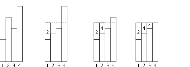
This is Walker’s alias method.

A complete description is in Ripley (1987, Alg 3.13B).

The alias method is an example of trading off a setup cost for fast generation.

The alias method is used by the sample function for unequal probability sampling with replacement when there are enough reasonably probable values. (source code in svn)

9.4.4 Accept/Reject Methods

9.4.4.1 Sampling Uniformly from the Area Under a Density

Suppose \(h\) is a function such that

• \(h(x) \ge 0\) for all \(x\)
• \(\int h(x) dx < \infty\).

Let

\[\begin{equation*} \mathcal{G}_h = \{(x,y): 0 < y \le h(x)\} \end{equation*}\]

The area of \(\mathcal{G}_h\) is

\[\begin{equation*} |\mathcal{G}_h| = \int h(x) dx < \infty \end{equation*}\]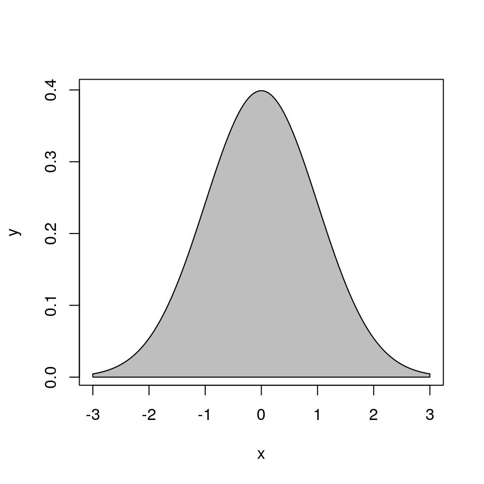

Suppose \((X,Y)\) is uniformly distributed on \(\mathcal{G}_h\). Then

• The conditional distribution of \(Y|X=x\) is uniform on \((0,h(x))\).

• The marginal distribution of \(X\) has density \(f_X(x) = h(x)/\int h(y) dy\): \[\begin{equation*} f_X(x) = \int_0^{h(x)}\frac{1}{|\mathcal{G}_h|} dy = \frac{h(x)}{\int h(y) dy} \end{equation*}\]

9.4.4.2 Rejection Sampling Using an Envelope Density

Suppose \(g\) is a density and \(M > 0\) is a real number such that

\[\begin{equation*} h(x) \le M g(x) \quad \text{for all $x$} \end{equation*}\]

or, equivalently,

\[\begin{equation*} \sup \frac{h(x)}{g(x)} \le M \quad \text{for all $x$} \end{equation*}\]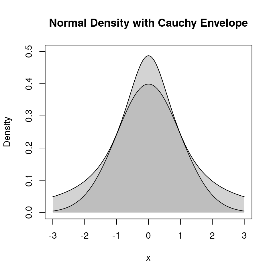

\(M g(x)\) is an envelope for \(h(x)\).

Suppose

• we want to sample from a density proportional to \(h\);

• we can find a density \(g\) and a constant \(M\) such that

  • \(M g(x)\) is an envelope for \(h(x)\);
  • it is easy to sample from \(g\).

Then

• we can sample \(X\) from \(g\) and \(Y|X=x\) from \(\text{U}(0,Mg(x))\) to get a pair \((X,Y)\) uniformly distributed on \(\mathcal{G}_{Mg}\);

• we can repeat until the pair \((X,Y)\) satisfies \(Y \le h(X)\).

The resulting pair \((X,Y)\) is uniformly distributed on \(\mathcal{G}_h\);

Therefore the marginal density of the resulting \(X\) is \(f_X(x) = h(x)/\int h(y) dy\).

The number of draws from the uniform distribution on \(\mathcal{G}_{Mg}\) needed until we obtain a pair in \(\mathcal{G}_h\) is independent of the final pair.

The number of draws has a geometric distribution with success probability

\[\begin{equation*} p = \frac{|\mathcal{G}_h|}{|\mathcal{G}_{Mg}|} = \frac{\int h(y) dy}{M \int g(y) dy} = \frac{\int h(y) dy}{M} \end{equation*}\]

since \(g\) is a probability density. \(p\) is the acceptance probability.

The expected number of draws needed is

\[\begin{equation*} E[\text{number of draws}] = \frac{1}{p} = \frac{M \int g(y) dy}{\int h(y) dy} = \frac{M}{\int h(y) dy}. \end{equation*}\]

If \(h\) is also a proper density, then \(p = 1/M\) and

\[\begin{equation*} E[\text{number of draws}] = \frac{1}{p} = M \end{equation*}\]

9.4.4.3 The Basic Algorithm

The rejection, or accept/reject, sampling algorithm:

   repeat        Generate independent \(X \sim g\) and \(U \sim \text{U}[0,1]\)    until \(U M g(X) \le h(X)\)    return \(X\)

Alternate forms of the test:

\[\begin{align*} U &\le \frac{h(X)}{M g(X)}\\ \log(U) &\le \log(h(X)) - \log(M) - \log(g(X)) \end{align*}\]

Care may be needed to ensure numerical stability.

9.4.4.4 Example: Normal Distribution with Cauchy Envelope

Suppose

• \(h(x) = \frac{1}{\sqrt{2\pi}} e^{-x^2/2}\) is the standard normal density
• \(g(x) = \frac{1}{\pi(1 + x^2)}\) is the standard Cauchy density

Then

\[\begin{equation*} \frac{h(x)}{g(x)} = \sqrt{\frac{\pi}{2}} (1+x^2)e^{-x^2/2} \le \sqrt{\frac{\pi}{2}} (1+1^2)e^{-1^2/2} = \sqrt{2\pi e^{-1}} = 1.520347 \end{equation*}\]

The resulting accept/reject algorithm is

   repeat        Generate independent standard Cauchy \(X\) and \(U \sim \text{U}[0,1]\)    until \(U \le \frac{e^{1/2}}{2}(1+X^2)e^{-X^2/2}\)    return \(X\)

9.4.4.5 Squeezing

Performance can be improved by squeezing:

Accept if point is inside the triangle:

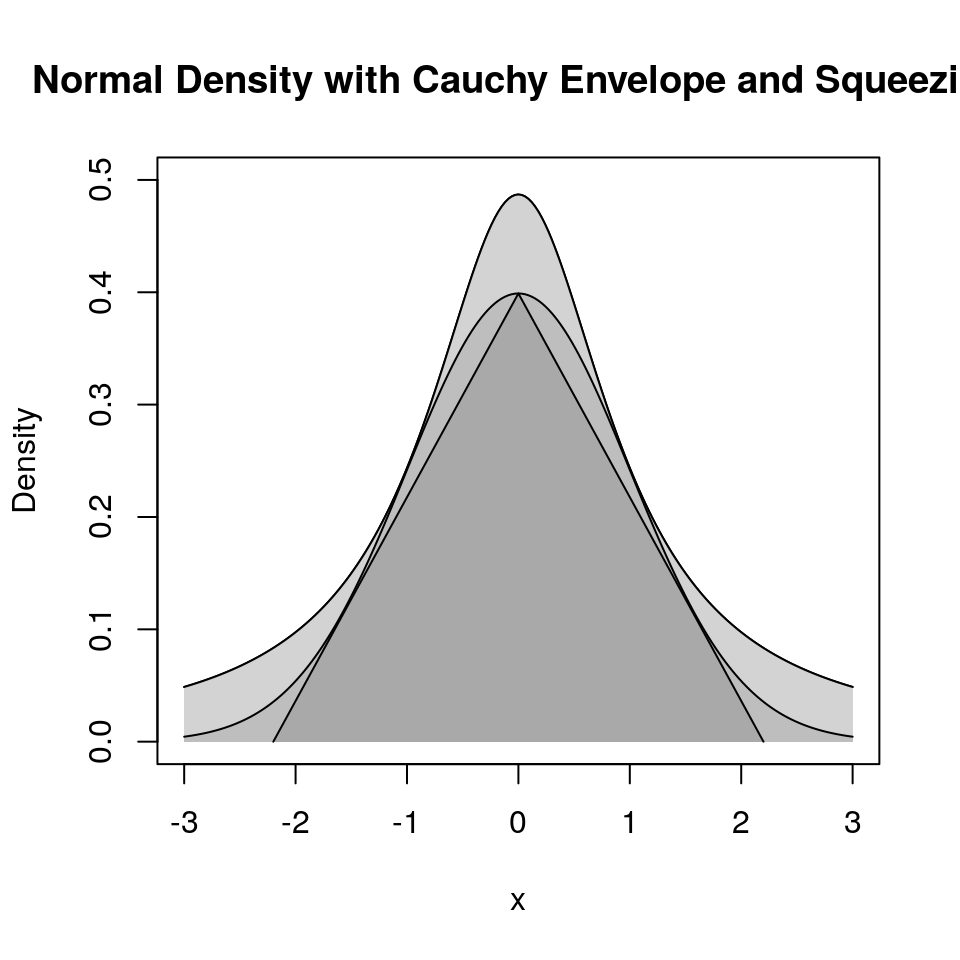
Squeezing can speed up generation.

Squeezing will complicate the code (making errors more likely).

9.4.4.6 Rejection Sampling for Discrete Distributions

For simplicity, just consider integer valued random variables.

• If \(h\) and \(g\) are probability mass functions on the integers and \(h(x)/g(x)\) is bounded, then the same algorithm can be used.

• If \(p\) is a probability mass function on the integers then

  \[\begin{equation*} h(x) = p(\lfloor x \rfloor) \end{equation*}\]

  is a probability density.

• If \(X\) has density \(h\), then \(Y = \lfloor X \rfloor\) has PMF \(p\).

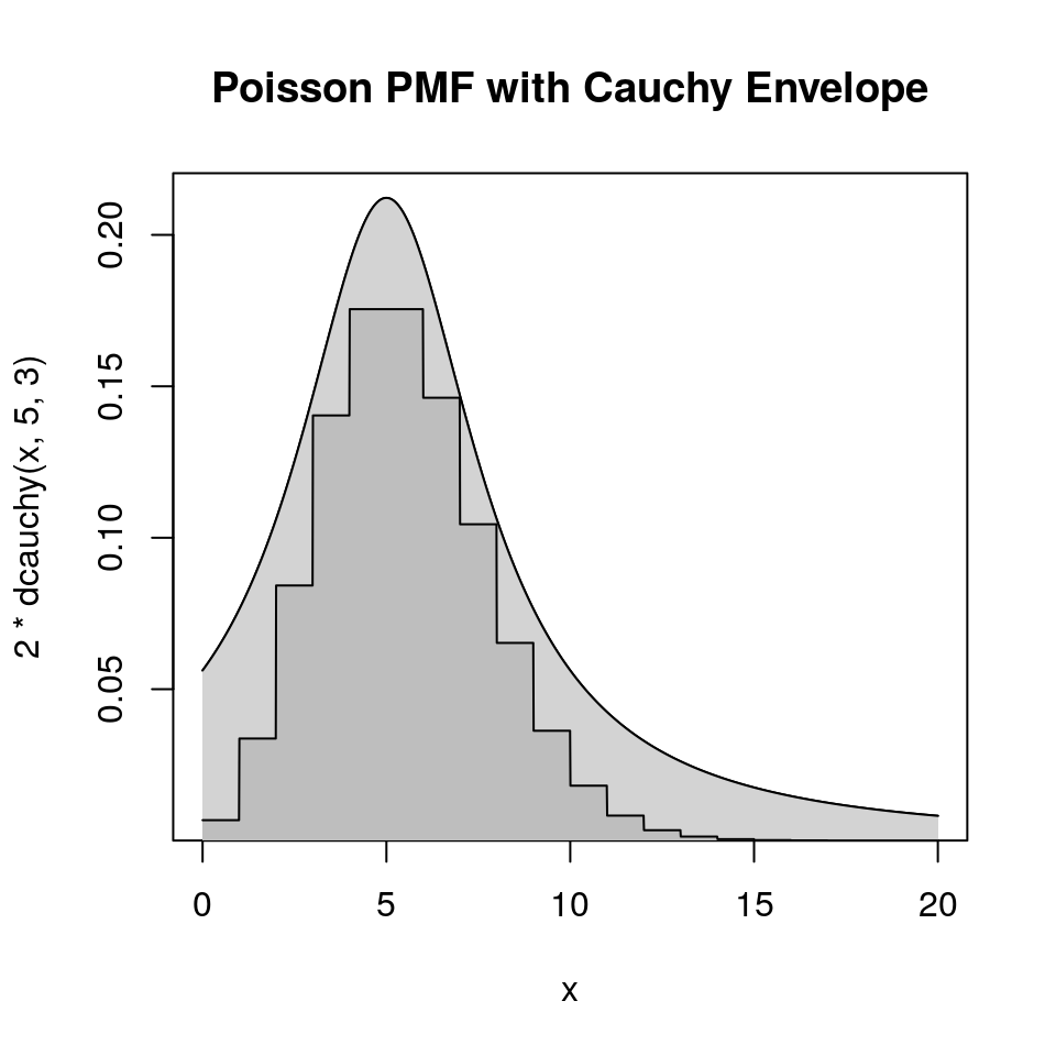
9.4.4.7 Example: Poisson Distribution with Cauchy Envelope

Suppose

• \(p\) is the PMF of a Poisson distribution with mean 5
• \(g\) is the Cauchy density with location 5 and scale 3.
• \(h(x) = p(\lfloor x \rfloor)\)

Then, by careful analysis or graphical examination, \(h(x) \le 2 g(x)\) for all \(x\).

9.4.4.8 Comments

The Cauchy density is often a useful envelope.

More efficient choices are often possible.

Location and scale need to be chosen appropriately.

If the target distribution is non-negative, a truncated Cauchy can be used.

Careful analysis is needed to produce generators for a parametric family (e.g. all Poisson distributions).

Graphical examination can be very helpful in guiding the analysis.

Carefully tuned envelopes combined with squeezing can produce very efficient samplers.

Errors in tuning and squeezing will produce garbage.

9.4.5 Ratio-of-Uniforms Method

9.4.5.1 Basic Method

Introduced by Kinderman and Monahan (1977).

Suppose

• \(h(x) \ge 0\) for all \(x\)
• \(\int h(x) dx < \infty\)

Let \((V, U)\) be uniform on

\[\begin{equation*} \mathcal{C}_h = \{(v,u): 0 < u \le \sqrt{h(v/u)}\} \end{equation*}\]

Then \(X = V/U\) has density \(f(x) = h(x)/\int h(y) dy\).

For \(h(x) = e^{-x^2/2}\) the region \(\mathcal{C}_h\) looks like

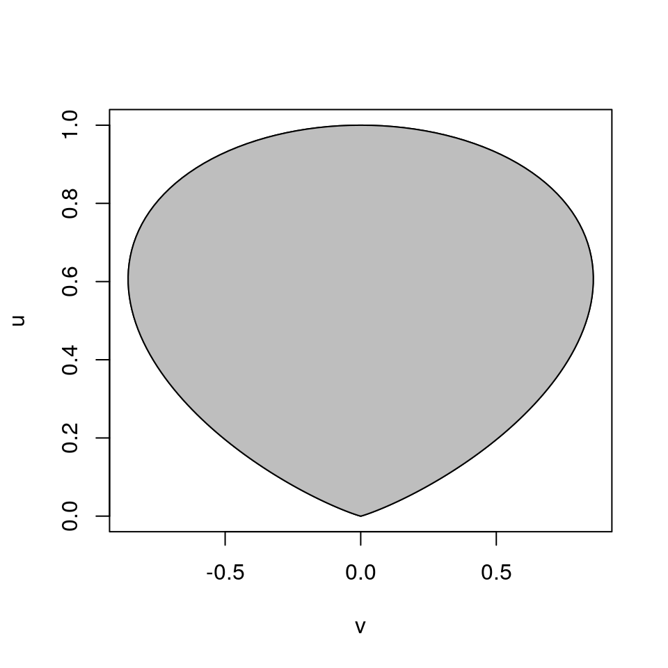
In this example:

• The region is bounded.

• The region is convex.

9.4.5.2 Properties

The region \(\mathcal{C}_h\) is convex if \(h\) is log concave.

The region \(\mathcal{C}_h\) is bounded if \(h(x)\) and \(x^2 h(x)\) are bounded.

Let

\[\begin{align*} u^* &= \max_x \sqrt{h(x)}\\ v_-^* &= \min_x x \sqrt{h(x)}\\ v_+^* &= \max_x x \sqrt{h(x)} \end{align*}\]

Then \(\mathcal{C}_h\) is contained in the rectangle \([v_-^*,v_+^*]\times[0,u^*]\).

The simple Ratio-of-Uniforms algorithm based on rejection sampling from the enclosing rectangle is

   repeat        Generate \(U \sim \text{U}[0,u^*]\)        Generate \(V \sim \text{U}[v_-^*,v_+^*]\)    until \(U^2 \le h(V/U)\)    return \(X = V/U\)

If \(h = e^{-x^2/2}\) then \[\begin{align*} u^* &= 1\\ v_-^* &= -\sqrt{2e^{-1}}\\ v_+^* &= \sqrt{2e^{-1}} \end{align*}\]

and the expected number of draws is

\[\begin{equation*} \frac{\text{area of rectangle}}{\text{area of $\mathcal{C}_h$}} = \frac{u^*(v_+^*-v_-^*)}{\frac{1}{2}\int h(x)dx} = \frac{2\sqrt{2e^{-1}}}{\sqrt{\pi/2}} = 1.368793 \end{equation*}\]

Various squeezing methods are possible.

Other approaches to sampling from \(\mathcal{C}_h\) are also possible.

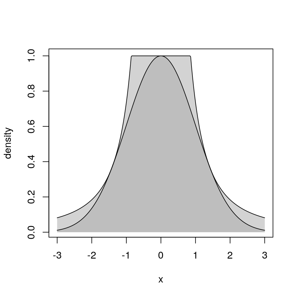
9.4.5.3 Relation to Rejection Sampling

Ratio of Uniforms with rejection sampling from the enclosing rectangle is equivalent to ordinary rejection sampling using an envelope density

\[\begin{equation*} g(x) \propto \begin{cases} \left(\frac{v_-^*}{x}\right)^2 & \text{if $x < v_-^*/u^*$}\\ (u^*)^2 & \text{if $v_-^*/u^* \le x \le v_+^*/u^*$}\\ \left(\frac{v_+^*}{x}\right)^2 & \text{if $x > v_+^*/u^*$} \end{cases} \end{equation*}\]

This is sometimes called a table mountain density

9.4.5.4 Generalizations

A more general form of the basic result: For any \(\mu\) and any \(r > 0\) let

\[\begin{equation*} \mathcal{C}_{h,\mu, r} = \{(v,u): 0 < u \le h(v/u^r+\mu)^{1/(r+1)}\} \end{equation*}\]

If \((U,V)\) is uniform on \(\mathcal{C}_{h,\mu, r}\), then \(X = V/U^r + \mu\) has density \(f(x) = h(x)/\int h(y)dy\).

• \(\mu\) and \(r\) can be chosen to minimize the rejection probability.

• \(r = 1\) seems adequate for most purposes.

• Choosing \(\mu\) equal to the mode of \(h\) can help.

• For the Gamma distribution with \(\alpha = 30\),

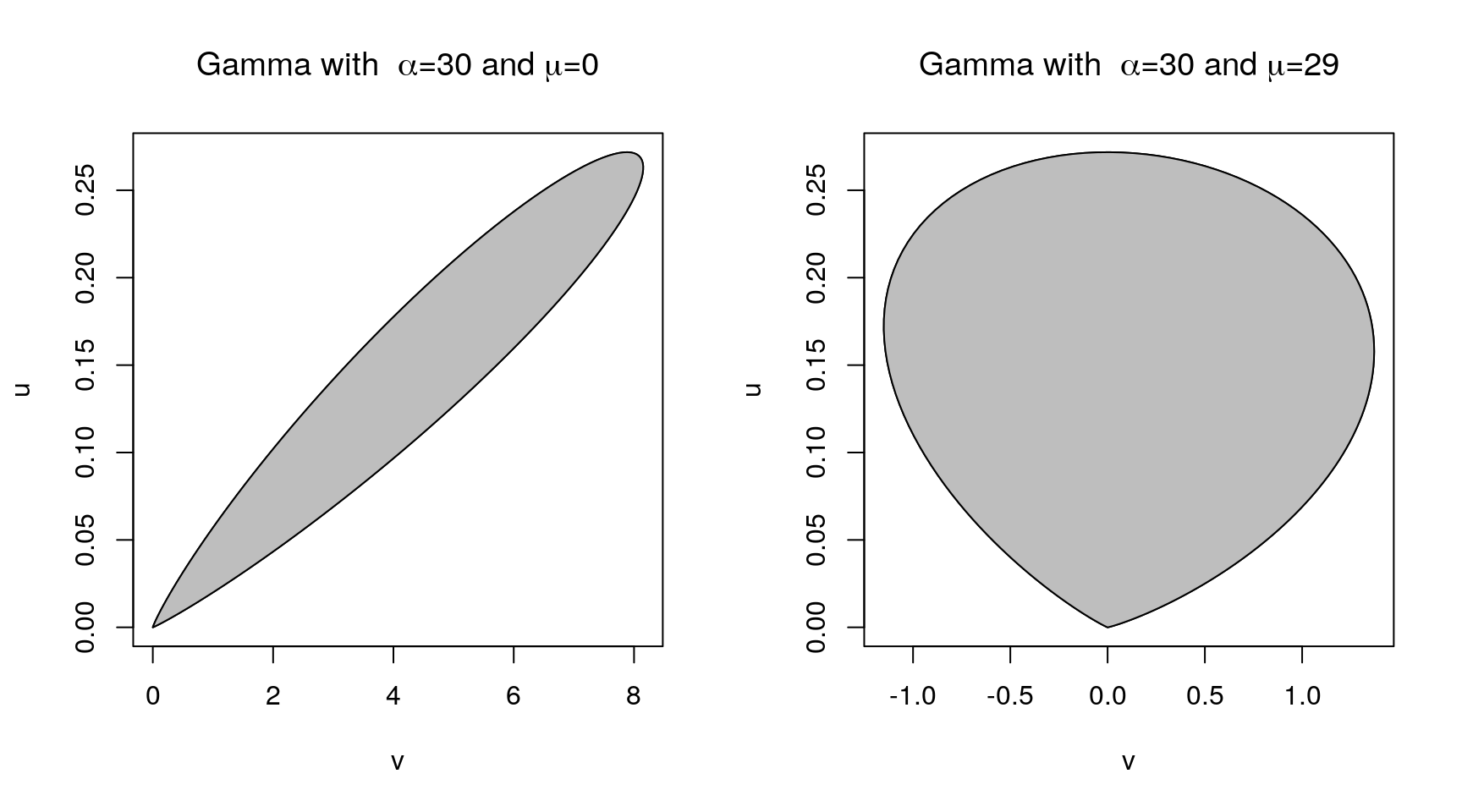
9.4.6 Adaptive Rejection Sampling

First introduced by Gilks and Wild (1992).

9.4.6.1 Convexity

A set \(C\) is convex if \(\lambda x + (1-\lambda)y \in C\) for all \(x, y \in C\) and \(\lambda \in [0, 1]\).

\(C\) can be a subset or \({\mathbb{R}}\), or \({\mathbb{R}}^n\), or any other set where the convex combination

\[\begin{equation*} \lambda x + (1-\lambda)y \end{equation*}\]

makes sense.

A real-valued function \(f\) on a convex set \(C\) is convex if

\[\begin{equation*} f(\lambda x + (1 - \lambda) y) \le \lambda f(x) + (1-\lambda) f(y) \end{equation*}\]

\(x, y \in C\) and \(\lambda \in [0, 1]\).

\(f(x)\) is concave if \(-f(x)\) is convex, i.e. if

\[\begin{equation*} f(\lambda x + (1 - \lambda) y) \ge \lambda f(x) + (1-\lambda) f(y) \end{equation*}\]

\(x, y \in C\) and \(\lambda \in [0, 1]\).

A concave function is always below its tangent.

9.4.6.2 Log Concave Densities

A density \(f\) is log concave if \(\log f\) is a concave function

Many densities are log concave:

• normal densities;

• Gamma(\(\alpha,\beta\)) with \(\alpha \ge 1\);

• Beta(\(\alpha,\beta\)) with \(\alpha \ge 1\) and \(\beta \ge 1\).

Some are not but may be related to ones that are: The \(t\) densities are not, but if

\[\begin{align*} X|Y=y &\sim \text{N}(0,1/y)\\ Y &\sim \text{Gamma}(\alpha, \beta) \end{align*}\]

then

• the marginal distribution of \(X\) is \(t\) for suitable choice of \(\beta\)

• and the joint distribution of \(X\) and \(Y\) has density \[\begin{equation*} f(x,y) \propto \sqrt{y}e^{-\frac{y}{2}x^2}y^{\alpha-1}e^{-y/\beta} = y^{\alpha-1/2}e^{-y(\beta+x^2/2)} \end{equation*}\]

  which is log concave for \(\alpha \ge 1/2\)

9.4.6.3 Tangent Approach

Suppose

• \(f\) is log concave;
• \(f\) has an interior mode

Need log density, derivative at two points, one each side of the mode

• piece-wise linear envelope of log density
• piece-wise exponential envelope of density
• if first point is not accepted, can use to make better envelope

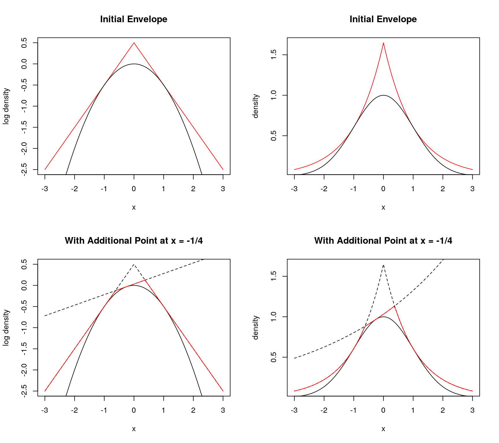
9.4.6.4 Secant Approach

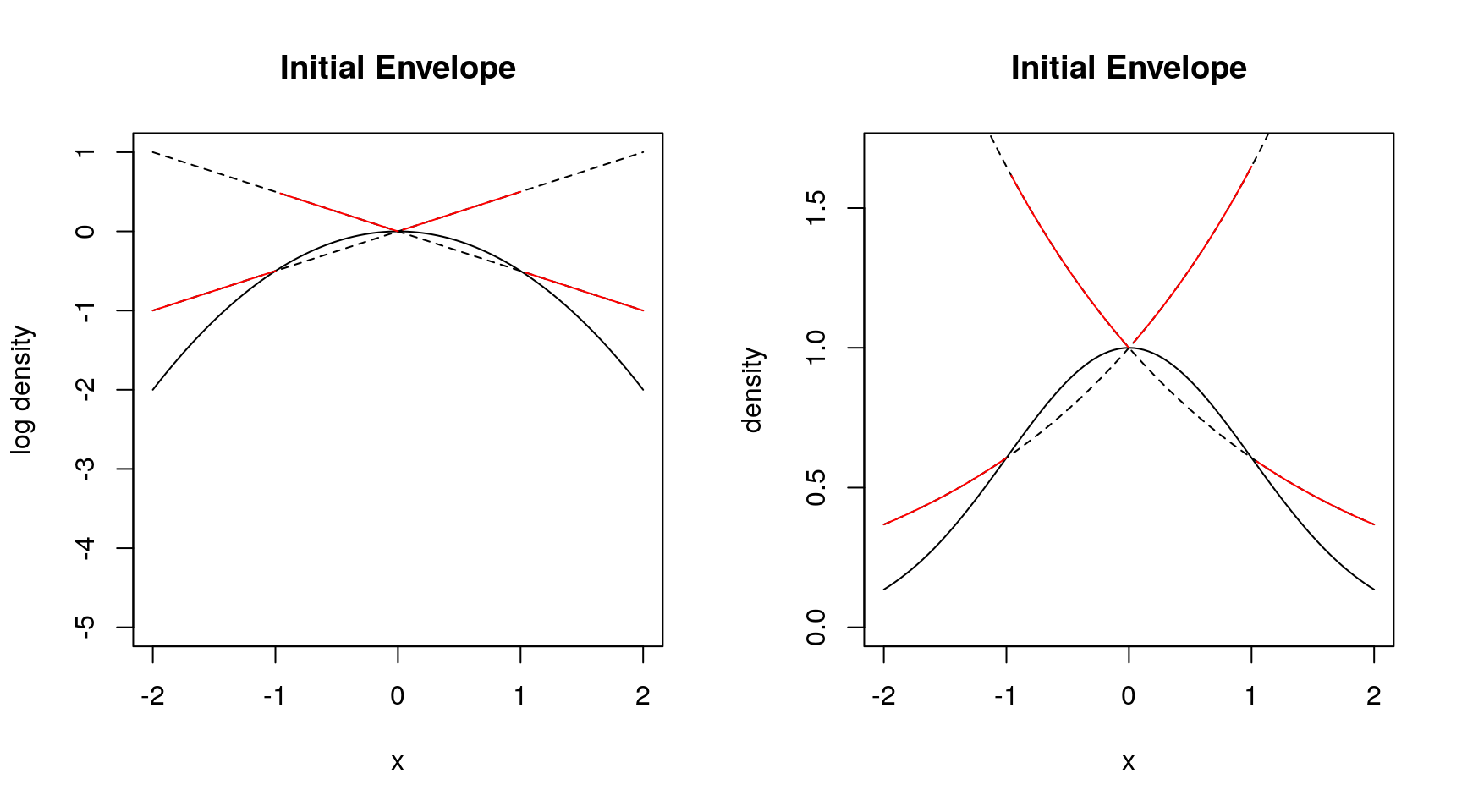
• Need three points to start
• Do not need derivatives
• Get larger rejection rates

Both approaches need numerical care

9.4.7 Notes and Comments

Many methods depend on properties of a particular distribution.

Inversion is one general method that can often be used.

Other general-purpose methods are

• rejection sampling;
• adaptive rejection sampling;
• ratio-of-uniforms.

Some references:

• Devroye, L. (1986). Non-Uniform Random Variate Generation, Springer-Verlag, New York.

• Gentle, J. E. (2003). Random Number Generation and Monte Carlo Methods, Springer-Verlag, New York.

• Hoermann, W., Leydold, J., and Derflinger, G. (2004). Automatic Nonuniform Random Variate Generation, Springer-Verlag, New York.

A Recent Publication:

• Karney, C.F.F. (2016). ``Sampling Exactly from the Normal Distribution.’’ ACM Transactions on Mathematical Software 42 (1).

9.4.8 Random Variate Generators in R

Generators for most standard distributions are available

• rnorm: normal
• rgamma: gamma
• rt: \(t\)
• rpois: Poisson
• etc.

Most use standard algorithms from the literature.

Source code is in src/nmath/ in the source tree.

The normal generator can be configured by RNGkind. Options are

• Kinderman-Ramage
• Buggy Kinderman-Ramage (available for reproducing results)
• Ahrens-Dieter
• Box-Muller
• Inversion (the current default)
• user-supplied

9.5 Generating Random Vectors and Matrices

Sometimes generating random vectors can be reduced to a series of univariate generations.

One approach is conditioning: \[\begin{equation*} f(x,y,z) = f_{Z|X,Y}(z|x,y) f_{Y|X}(y|x) f_X(x) \end{equation*}\]

So we can generate

• \(X\) from \(f_X(x)\)
• \(Y|X=x\) from \(f_{Y|X}(y|x)\)
• \(Z|X=x,Y=y\) from \(f_{Z|X,Y}(z|x,y)\)

One example: \((X_1,X_2,X_3) \sim \text{Multinomial}(n,p_1,p_2,p_3)\). Then

\[\begin{align*} X_1 &\sim \text{Binomial}(n, p_1)\\ X_2 | X_1 = x_1 &\sim \text{Binomial}(n - x_1, p_2/(p_2+p_3))\\ X_3 | X_1 = x_1, X_2 = x_2 &= n - x_1 - x_2 \end{align*}\]

Another example: \(X, Y\) bivariate normal \((\mu_X, \mu_Y, \sigma_X^2, \sigma_Y^2, \rho)\). Then

\[\begin{align*} X &\sim \text{N}(\mu_X,\sigma_X^2)\\ Y|X=x &\sim \text{N}\left(\mu_Y + \rho\frac{\sigma_Y}{\sigma_X}(x-\mu_X), \sigma_Y^2(1-\rho^2)\right) \end{align*}\]

For some distributions special methods are available.

Some general methods extend to multiple dimensions.

9.5.1 Multivariate Normal Distribution

Marginal and conditional distributions are normal; conditioning can be used in general.

Alternative: use linear transformations.

Suppose \(Z_1, \dots, Z_d\) are independent standard normals, \(\mu_1, \dots \mu_d\) are constants, and \(A\) is a constant \(d \times d\) matrix. Let

\[\begin{align*} Z &= \ \begin{bmatrix} Z_1\\ \vdots\\ Z_d \end{bmatrix} & \mu &= \begin{bmatrix} \mu_1\\ \vdots\\ \mu_d \end{bmatrix} \end{align*}\]

and set

\[\begin{equation*} X = \mu + A Z \end{equation*}\]

Then \(X\) is multivariate normal with mean vector \(\mu\) and covariance matrix \(A A^T\),

\[\begin{equation*} X \sim \text{MVN}_d(\mu, A A^T) \end{equation*}\]

To generate \(X \sim \text{MVN}_d(\mu, \Sigma)\), we can

• find a matrix \(A\) such that \(A A^T = \Sigma\)
• generate elements of \(Z\) as independent standard normals
• compute \(X = \mu + A Z\)

The Cholesky factorization is one way to choose \(A\).

If we are given \(\Sigma^{-1}\), then we can

• decompose \(\Sigma^{-1} = L L^T\)
• solve \(L^T Y = Z\)
• compute \(X = \mu + Y\)

9.5.2 Spherically Symmetric Distributions

A joint distribution is called spherically symmetric (about the origin) if it has a density of the form

\[\begin{equation*} f(x) = g(x^T x) = g(x_1^2 + \dots + x_d^2). \end{equation*}\]

If the distribution of \(X\) is spherically symmetric then

\[\begin{align*} R &= \sqrt{X^T X}\\ Y &= X/R \end{align*}\]

are independent,

• \(Y\) is uniformly distributed on the surface of the unit sphere.
• \(R\) has density proportional to \(g(r)r^{d-1}\) for \(r > 0\).

We can generate \(X \sim f\) by

• generating \(Z \sim \text{MVN}_d(0, I)\) and setting \(Y = Z /\sqrt{Z^T Z}\)

• generating \(R\) from the density proportional to \(g(r)r^{d-1}\) by univariate methods.

9.5.3 Elliptically Contoured Distributions

A density \(f\) is elliptically contoured if \[\begin{equation*} f(x) = \frac{1}{\sqrt{\det \Sigma}} g((x-\mu)^T\Sigma^{-1}(x-\mu)) \end{equation*}\]

for some vector \(\mu\) and symmetric positive definite matrix \(\Sigma\).

Suppose \(Y\) has spherically symmetric density \(g(y^Ty)\) and \(A A^T = \Sigma\). Then \(X = \mu + A Y\) has density \(f\).

9.5.4 Wishart Distribution

Suppose \(X_1, \dots X_n\) are independent and \(X_i \sim \text{MVN}_d(\mu_i,\Sigma)\). Let

\[\begin{equation*} W = \sum_{i=1}^{n} X_i X_i^T \end{equation*}\]

Then \(W\) has a non-central Wishart distribution \(\text{W}(n, \Sigma, \Delta)\) where \(\Delta = \sum \mu_i\mu_i^T\).

If \(X_i \sim \text{MVN}_d(\mu,\Sigma)\) and

\[\begin{equation*} S = \frac{1}{n-1}\sum_{i=1}^n (X_i -\overline{X})(X_i -\overline{X})^T \end{equation*}\]

is the sample covariance matrix, then \((n-1) S \sim \text{W}(n-1, \Sigma, 0)\).

Suppose \(\mu_i = 0\), \(\Sigma = A A^T\), and \(X_i = A Z_i\) with \(Z_i \sim \text{MVN}_d(0,I)\). Then \(W = AVA^T\) with

\[\begin{equation*} V = \sum_{i=1}^n Z_i Z_i^T \end{equation*}\]

Bartlett decomposition: In the Cholesky factorization of \(V\)

• all elements are independent;
• the elements below the diagonal are standard normal;
• the square of the \(i\)-th diagonal element is \(\chi^2_{n+1-i}\).

If \(\Delta \neq 0\) let \(\Delta = B B^T\) be its Cholesky factorization, let \(b_i\) be the columns of \(B\) and let \(Z_1,\dots,Z_n\) be independent \(\text{MVN}_d(0,I)\) random vectors. Then for \(n \ge d\)

\[\begin{equation*} W = \sum_{i=1}^d(b_i + A Z_i)(b_i + A Z_i)^T + \sum_{i=d+1}^n A Z_i Z_i^T A^T \sim \text{W}(n, \Sigma, \Delta) \end{equation*}\]

9.5.5 Rejection Sampling

Rejection sampling can in principle be used in any dimension.

A general envelope that is sometimes useful is based on generating \(X\) as

\[\begin{equation*} X = b + A Z/Y \end{equation*}\]

where

• \(Z\) and \(Y\) are independent
• \(Z \sim \text{MVN}_d(0, I)\)
• \(Y^2 \sim \text{Gamma}(\alpha, 1/\alpha)\), a scalar
• \(b\) is a vector of constants
• \(A\) is a matrix of constants

This is a kind of multivariate \(t\) random vector.

This often works in modest dimensions.

Specially tailored envelopes can sometimes be used in higher dimensions.

Without special tailoring, rejection rates tend to be too high to be useful.

9.5.6 Ratio of Uniforms

The ratio-of-uniforms method also works in \({\mathbb{R}}^d\): Suppose

• \(h(x) \ge 0\) for all \(x\)
• \(\int h(x) dx < \infty\)

Let

\[ \mathcal{C}_h = \{(v,u): v \in {\mathbb{R}}^d, 0 < u \le \sqrt[d+1]{h(v/u + \mu)}\} \]

for some \(\mu\). If \((V,U)\) is uniform on \(\mathcal{C}_h\), then \(X = V/U+\mu\) has density \(f(x) = h(x)/\int h(y) dy\).

If \(h(x)\) and \({\|{x}\|}^{d+1}h(x)\) are bounded, then \(\mathcal{C}_h\) is bounded.

If \(h(x)\) is log concave then \(\mathcal{C}_h\) is convex.

Rejection sampling from a bounding hyper rectangle works in modest dimensions.

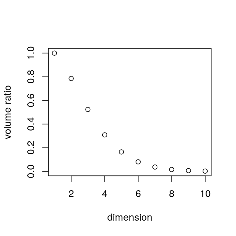
It will not work for dimensions larger than 8 or so:

• The shape of \(\mathcal{C}_h\) is vaguely spherical.

• The volume of the unit sphere in \(d\) dimensions is \[\begin{equation*} V_d = \frac{\pi^{d/2}}{\Gamma(d/2 + 1)} \end{equation*}\]

• The ratio of this volume to the volume of the enclosing hyper cube, \(2^d\) tends to zero very fast:

9.5.7 Order Statistics

The order statistics for a random sample \(X_1,\dots,X_n\) from \(F\) are the ordered values

\[\begin{equation*} X_{(1)} \le X_{(2)} \le \dots \le X_{(n)} \end{equation*}\]

• We can simulate them by ordering the sample.

• Faster \(O(n)\) algorithms are available for individual order statistics, such as the median.

If \(U_{(1)} \le \dots \le U_{(n)}\) are the order statistics of a random sample from the \(\text{U}[0,1]\) distribution, then

\[\begin{align*} X_{(1)} &= F^-(U_{(1)})\\ &\;\;\vdots\\ X_{(n)} &= F^-(U_{(n)}) \end{align*}\]

are the order statistics of a random sample from \(F\).

For a sample of size \(n\) the marginal distribution of \(U_{(k)}\) is

\[\begin{equation*} U_{(k)} \sim \text{Beta}(k, n-k+1). \end{equation*}\]

Suppose \(k < \ell\).

• Then \(U_{(k)}/U_{(\ell)}\) is independent of \(U_{(\ell)}, \dots, U_{(n)}\)

• \(U_{(k)}/U_{(\ell)}\) has a \(\text{Beta}(k, \ell-k)\) distribution.

We can use this to generate any subset or all order statistics.

Let \(V_1, \dots, V_{n+1}\) be independent exponential random variables with the same mean and let

\[\begin{equation*} W_k = \frac{V_1+\dots+V_k}{V_1+\dots+V_{n+1}} \end{equation*}\]

Then \(W_1, \dots, W_n\) has the same joint distribution as \(U_{(1)}, \dots, U_{(n)}\).

9.5.8 Homogeneous Poisson Process

For a homogeneous Poisson process with rate \(\lambda\)

• The number of points \(N(A)\) in a set \(A\) is Poisson with mean \(\lambda|A|\).

• If \(A\) and \(B\) are disjoint then \(N(A)\) and \(N(B)\) are independent.

Conditional on \(N(A) = n\), the \(n\) points are uniformly distributed on \(A\).

We can generate a Poisson process on \([0,t]\) by generating exponential variables \(T_1, T_2,\dots\) with rate \(\lambda\) and computing

\[\begin{equation*} S_k = T_1+\dots+T_k \end{equation*}\]

until \(S_k > t\). The values \(S_1, \dots, S_{k-1}\) are the points in the Poisson process realization.

9.5.9 Inhomogeneous Poisson Processes

For an inhomogeneous Poisson process with rate \(\lambda(x)\)

• The number of points \(N(A)\) in a set \(A\) is Poisson with mean \(\int_A\lambda(x) dx\).

• If \(A\) and \(B\) are disjoint then \(N(A)\) and \(N(B)\) are independent.

Conditional on \(N(A) = n\), the \(n\) points in \(A\) are a random sample from a distribution with density \(\lambda(x)/\int_A\lambda(y)dy\).

To generate an inhomogeneous Poisson process on \([0,t]\) we can

• Let \(\Lambda(s) = \int_0^s\lambda(x)dx\).

• Generate arrival times \(S_1, \dots, S_N\) for a homogeneous Poisson process with rate one on \([0,\Lambda(t)]\).

• Compute arrival times of the inhomogeneous process as \[\begin{equation*} \Lambda^{-1}(S_1),\dots,\Lambda^{-1}(S_N). \end{equation*}\]

If \(\lambda(x) \le M\) for all \(x\), then we can generate an inhomogeneous Poisson process with rate \(\lambda(x)\) by thinning:

• Generate a homogeneous Poisson process with rate \(M\) to obtain points \(X_1, \dots, X_N\).

• Independently delete each point \(X_i\) with probability \(1-\lambda(X_i)/M\).

The remaining points form a realization of an inhomogeneous Poisson process with rate \(\lambda(x)\).

If \(N_1\) and \(N_2\) are independent inhomogeneous Poisson processes with rates \(\lambda_1(x)\) and \(\lambda_2(x)\), then their superposition \(N_1+N_2\) is an inhomogeneous Poisson process with rate \(\lambda_1(x)+\lambda_2(x)\).

9.5.10 Other Processes

Many other processes can be simulated from their definitions

• Cox processes (doubly stochastic Poisson process)
• Poisson cluster processes
• ARMA, ARIMA processes
• GARCH processes

Continuous time processes, such as Brownian motion and diffusions, require discretization of time.

Other processes may require Markov chain methods

• Ising models
• Strauss process
• interacting particle systems

9.6 Variance Reduction

Most simulations involve estimating integrals or expectations: \[\begin{align*} \theta &= \int h(x) f(x) dx & \text{mean}\\ \theta &= \int 1_{\{X \in A\}} f(x) dx & \text{probability}\\ \theta &= \int (h(x) - E[h(X)])^2 f(x) dx & \text{variance}\\ &\;\;\vdots \end{align*}\]

The crude simulation, or crude Monte Carlo, or na"ive Monte Carlo, approach:

• Sample \(X_1,\dots,X_N\) independently from \(f\)

• Estimate \(\theta\) by \(\widehat{\theta}_N = \frac{1}{N} \sum h(X_i)\).

If \(\sigma^2 = {\text{Var}}(h(X))\), then \({\text{Var}}(\widehat{\theta}_N) = \frac{\sigma^2}{N}\).

To reduce the error we can:

• Increase \(N\): requires CPU time and clock time; diminishing returns.

• try to reduce \(\sigma^2\): requires thinking time, programming effort.

Methods that reduce \(\sigma^2\) are called

• tricks;
• swindles;
• Monte Carlo methods.

9.6.1 Control Variates

Suppose we have a random variable \(Y\) with mean \(\theta\) and a correlated random variable \(W\) with known mean \(E[W]\). Then for any constant \(b\)

\[\begin{equation*} \widetilde{Y} = Y - b(W-E[W]) \end{equation*}\]

has mean \(\theta\).

• \(W\) is called a control variate.

• Choosing \(b=1\) often works well if the correlation is positive and \(\theta\) and \(E[W]\) are close.

• The value of \(b\) that minimizes the variance of \(\widetilde{Y}\) is \({\text{Cov}}(Y,W)/{\text{Var}}(W)\).

• We can use a guess or a pilot study to estimate \(b\).

• We can also estimate \(b\) from the same data used to compute \(Y\) and \(W\).

• This is related to the regression estimator in sampling.

9.6.1.1 Example

Suppose we want to estimate the expected value of the sample median \(T\) for a sample of size 10 from a \(\text{Gamma}(3,1)\) population.

Crude estimate:

\[\begin{equation*} Y = \frac{1}{N}\sum T_i \end{equation*}\]

Using the sample mean as a control variate with \(b=1\):

\[\begin{equation*} \widehat{Y} = \frac{1}{N}\sum (T_i-\overline{X}_i) + E[\overline{X}_i] = \frac{1}{N}\sum (T_i-\overline{X}_i) + \alpha \end{equation*}\]

x <- matrix(rgamma(10000, 3), ncol = 10)
md <- apply(x, 1, median)
mn <- apply(x, 1, mean)
mean(md)
## [1] 2.738521
mean(md - mn) + 3
## [1] 2.725689
sd(md)
## [1] 0.6269172
sd(md-mn)
## [1] 0.3492994

The standard deviation is cut roughly in half.

The optimal \(b\) seems close to 1.

9.6.1.2 Control Variates and Probability Estimates

Suppose \(T\) is a test statistic and we want to estimate \(\theta = P(T \le t)\).

Crude Monte Carlo:

\[\begin{equation*} \widehat{\theta} = \frac{\#\{T_i \le t\}}{N} \end{equation*}\]

Suppose \(S\) is ``similar’’ to \(T\) and \(P(S \le t)\) is known. Use

\[\begin{equation*} \widehat{\theta} = \frac{\#\{T_i \le t\} - \#\{S_i \le t\}}{N} + P(S \le t) = \frac{1}{N}\sum Y_i + P(S \le t) \end{equation*}\]

with \(Y_i = 1_{\{T_i \le t\}} - 1_{\{S_i \le t\}}\).

If \(S\) mimics \(T\), then \(Y_i\) is usually zero.

Could use this to calibrate

\[\begin{equation*} T = \frac{\text{median}}{\text{interquartile range}} \end{equation*}\]

for normal data using the \(t\) statistic.

9.6.2 Importance Sampling

Suppose we want to estimate

\[\begin{equation*} \theta = \int h(x) f(x) dx \end{equation*}\]

for some density \(f\) and some function \(h\).

Crude Mote Carlo samples \(X_1,\dots,X_N\) from \(f\) and uses

\[\begin{equation*} \widehat{\theta} = \frac{1}{N} \sum h(X_i) \end{equation*}\]

If the region where \(h\) is large has small probability under \(f\) then this can be inefficient.

Alternative: Sample \(X_1,\dots X_n\) from \(g\) that puts more probability near the ``important’’ values of \(x\) and compute

\[\begin{equation*} \widetilde{\theta} = \frac{1}{N}\sum h(X_i)\frac{f(X_i)}{g(X_i)} \end{equation*}\] Then, if \(g(x) > 0\) when \(h(x)f(x) \neq 0\), \[\begin{equation*} E[\widetilde{\theta}] = \int h(x) \frac{f(x)}{g(x)} g(x) dx = \int h(x) f(x) dx = \theta \end{equation*}\]

and

\[ {\text{Var}}(\widetilde{\theta}) = \frac{1}{N} \int \left(h(x)\frac{f(x)}{g(x)} - \theta\right)^2 g(x) dx = \frac{1}{N} \left( \int \left(h(x)\frac{f(x)}{g(x)}\right)^2 g(x) dx - \theta^2\right) \]

The variance is minimized by \(g(x) \propto |h(x)f(x)|\)

9.6.2.1 Importance Weights

Importance sampling is related to stratified and weighted sampling in sampling theory.

The function \(w(x) = f(x)/g(x)\) is called the weight function.

Alternative estimator:

\[\begin{equation*} \theta^* = \frac{\sum h(X_i) w(X_i)}{\sum w(X_i)} \end{equation*}\]

This is useful if \(f\) or \(g\) or both are unnormalized densities.

Importance sampling can be useful for computing expectations with respect to posterior distributions in Bayesian analyses.

Importance sampling can work very well if the weight function is bounded.

Importance sampling can work very poorly if the weight function is unbounded—it is easy to end up with infinite variances.

9.6.2.2 Computing Tail Probabilities

Suppose \(\theta = P(X \in R)\) for some region \(R\).

Suppose we can find \(g\) such that \(f(x)/g(x) < 1\) on \(R\). Then

\[\begin{equation*} \widetilde{\theta} = \frac{1}{N} \sum 1_R(X_i)\frac{f(X_i)}{g(X_i)} \end{equation*}\]

and

\[\begin{align*} \renewcommand{\Var}{\text{Var}} \Var(\widetilde{\theta}) &= \frac{1}{N}\left(\int_R \left(\frac{f(x)}{g(x)}\right)^2 g(x) dx - \theta^2\right)\\ &= \frac{1}{N}\left(\int_R \frac{f(x)}{g(x)} f(x) dx - \theta^2\right)\\ &< \frac{1}{N}\left(\int_R f(x) dx - \theta^2\right)\\ &= \frac{1}{N}(\theta-\theta^2) = \Var(\widehat{\theta}) \end{align*}\]

For computing \(P(X>2)\) where \(X\) has a standard Cauchy distribution we can use a shifted distribution:

y <- rcauchy(10000,3)
tt <- ifelse(y > 2, 1, 0) * dcauchy(y) / dcauchy(y,3)
mean(tt)
## [1] 0.146356
sd(tt)
## [1] 0.1605086

The asymptotic standard deviation for crude Monte Carlo is approximately

sqrt(mean(tt) * (1 - mean(tt)))
## [1] 0.3534627

A tilted density \(g(x) \propto f(x) e^{\beta x}\) can also be useful.

9.6.3 Antithetic Variates

Suppose \(S\) and \(T\) are two unbiased estimators of \(\theta\) with the same variance \(\sigma^2\) and correlation \(\rho\), and compute

\[\begin{equation*} V = \frac{1}{2}(S+T) \end{equation*}\]

Then

\[\begin{equation*} \Var(V) = \frac{\sigma^2}{4}(2+2\rho) = \frac{\sigma^2}{2}(1+\rho) \end{equation*}\]

Choosing \(\rho < 0\) reduces variance.

Such negatively correlated pairs are called antithetic variates.

Suppose we can choose between generating independent \(T_1,\dots,T_{N}\)

\[\begin{equation*} \widehat{\theta} = \frac{1}{N}\sum_{i=1}^N T_i \end{equation*}\]

or independent pairs \((S_1,T_1),\dots,(S_{N/2},T_{N/2})\) and computing

\[\begin{equation*} \widetilde{\theta} = \frac{1}{N} \sum_{i=1}^{N/2}(S_i+T_i) \end{equation*}\]

If \(\rho < 0\), then \({\text{Var}}(\widetilde{\theta}) < {\text{Var}}(\widehat{\theta})\).

If \(T = f(U)\), \(U \sim \text{U}[0,1]\), and \(f\) is monotone, then \(S = f(1-U)\) is negatively correlated with \(T\) and has the same marginal distribution.

If inversion is used to generate variates, computing \(T\) from \(U_1, \dots\) and \(S\) from \(1-U_1, \dots\) often works.

Some uniform generators provide an option in the seed to switch between returning \(U_i\) and \(1-U_i\).

9.6.3.1 Example

For estimating the expected value of the median for samples of size 10 from the \(\text{Gamma}(3,1)\) distribution:

u <- matrix(runif(5000), ncol = 10)
x1 <- qgamma(u, 3)
x2 <- qgamma(1 - u, 3)
md1 <- apply(x1, 1, median)
md2 <- apply(x2, 1, median)
sqrt(2) * sd((md1 + md2) / 2)
## [1] 0.1035287

Control variates helps further a bit but need \(b = 0.2\) or so.

mn1 <- apply(x1, 1, mean)
mn2 <- apply(x2, 1, mean)
sqrt(2) * sd((md1 + md2 - 0.2 * (mn1 + mn2)) / 2)
## [1] 0.09653593

9.6.4 Latin Hypercube Sampling

Suppose we want to compute

\[\begin{equation*} \theta = E[f(U_1,\dots,U_d)] \end{equation*}\]

with \((U_1,\dots,U_d)\) uniform on \([0,1]^d\).

For each \(i\)

• independently choose permutation \(\pi_i\) of \(\{1, \dots, N\}\)

• generate \(U_i^{(j)}\) uniformly on \([\pi_i(j)/N, (\pi_i(j)+1)/N]\).

For \(d = 2\) and \(N = 10\):

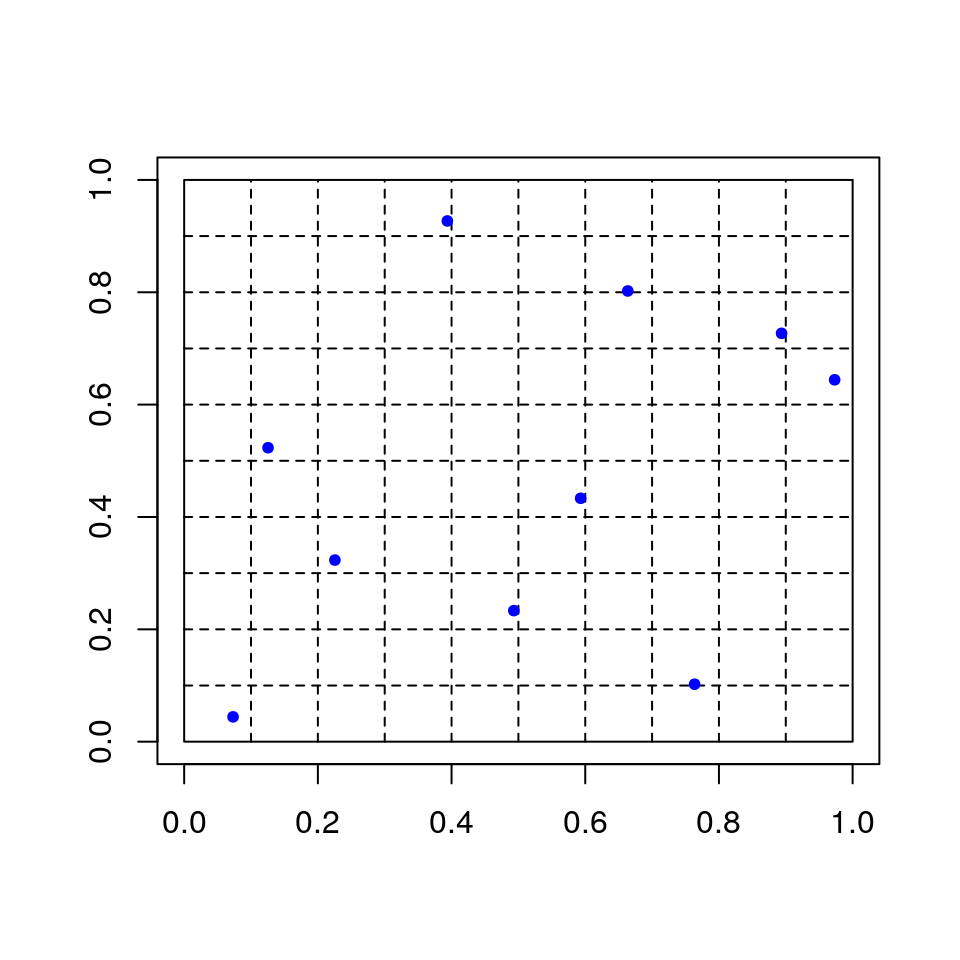
This is a random Latin square design.

In many cases this reduces variance compared to unrestricted random sampling (Stein, 1987; Avramidis and Wilson, 1995; Owen, 1992, 1998)

9.6.5 Common Variates and Blocking

Suppose we want to estimate \(\theta = E[S] - E[T]\)

One approach is to chose independent samples \(T_1,\dots,T_N\) and \(S_1,\dots,S_M\) and compute

\[\begin{equation*} \widehat{\theta} = \frac{1}{M}\sum_{i=1}^M S_i - \frac{1}{N}\sum_{i=1}^N T_i \end{equation*}\]

Suppose \(S = S(X)\) and \(T=T(X)\) for some \(X\). Instead of generating independent \(X\) values for \(S\) and \(T\) we may be able to

• use the common \(X\) values to generate pairs \((S_1,T_1),\dots,(S_N,T_N)\);

• compute \[\begin{equation*} \widetilde{\theta} = \frac{1}{N}\sum_{i=1}^N(S_i-T_i). \end{equation*}\]

This use of paired comparisons is a form of blocking.

This idea extends to comparisons among more than two statistics.

In simulations, we can often do this by using the same random variates to generate \(S_i\) and \(T_i\). This is called using common variates.

This is easiest to do if we are using inversion; this, and the ability to use antithetic variates, are two strong arguments in favor of inversion.

Using common variates may be harder when rejection-based methods are involved.

In importance sampling, using

\[\begin{equation*} \theta^* = \frac{\sum h(X_i)w(X_i)}{\sum w(X_i)} \end{equation*}\]

can be viewed as a paired comparison; for some forms of \(h\) is can have lower variance than the estimator that does not normalize by the sum of the weights.

9.6.6 Conditioning or Rao-Blackwellization

Suppose we want to estimate \(\theta = E[X]\)

If \(X, W\) are jointly distributed, then

\[\begin{equation*} \theta = E[X] = E[E[X|W]] \end{equation*}\]

and

\[\begin{equation*} \Var(X) = E[\Var(X|W)] + \Var(E[X|W]) \ge \Var(E[X|W]) \end{equation*}\]

Suppose we can compute \(E[X|W]\). Then we can

• generate \(W_1, \dots, W_N\);

• compute \[\begin{equation*} \widetilde{\theta} = \frac{1}{N} \sum E[X|W_i]. \end{equation*}\]

This is often useful in Gibbs sampling.

Variance reduction is not guaranteed if \(W_1,\dots,W_N\) are not independent.

Conditioning is particularly useful for density estimation: If we can compute \(f_{X|W}(x|w)\) and generate \(W_1,\dots,W_N\), then

\[\begin{equation*} \widehat{f}_X(x) = \frac{1}{N}\sum f_{X|W}(x|W_i) \end{equation*}\]

is much more accurate than, say, a kernel density estimate based on a sample \(X_1,\dots,X_N\).

9.6.6.1 Example

Suppose we want to estimate \(\theta = P(X > t)\) where \(X=Z/W\) with \(Z,W\) independent, \(Z \sim \text{N}(0,1)\) and \(W > 0\). Then

\[\begin{equation*} P(X>t|W=w) = P(Z > tw) = 1-\Phi(tw) \end{equation*}\]

So we can estimate \(\theta\) by generating \(W_1,\dots,W_N\) and computing

\[\begin{equation*} \widetilde{\theta} = \frac{1}{N}\sum (1 - \Phi(tW_i)) \end{equation*}\]

9.6.7 Independence Decomposition

Suppose \(X_1,\dots,X_n\) is a random sample from a \(\text{N}(0,1)\) distribution and

\[\begin{equation*} \widetilde{X} = \text{median}(X_1,\dots,X_n) \end{equation*}\]

We want to estimate \(\theta = {\text{Var}}(\widetilde{X}) = E[\widetilde{X}^2]\).

Crude Monte Carlo estimate: generate independent medians \(\widetilde{X}_1,\dots,\widehat{X}_N\) and compute

\[\begin{equation*} \widehat{\theta} = \frac{1}{N}\sum \widetilde{X}_i^2 \end{equation*}\]

Alternative: Write

\[\begin{equation*} \widetilde{X} = (\widetilde{X}-\overline{X})+\overline{X} \end{equation*}\]

\((\widetilde{X}-\overline{X})\) and \(\overline{X}\) are independent, for example by Basu’s theorem. So

\[\begin{equation*} E[\widetilde{X}^2|\overline{X}] = \overline{X}^2 + E[(\widetilde{X}-\overline{X})^2] \end{equation*}\]

and

\[\begin{equation*} \theta = \frac{1}{n} + E[(\widetilde{X}-\overline{X})^2] \end{equation*}\]

So we can estimate \(\theta\) by generating pairs \((\widetilde{X}_i,\overline{X}_i)\) and computing

\[\begin{equation*} \widetilde{\theta} = \frac{1}{n} + \frac{1}{N}\sum(\widetilde{X}_i-\overline{X}_i)^2 \end{equation*}\]

Generating these pairs may be more costly than generating medians alone.

9.6.7.1 Example

Estimates:

x <- matrix(rnorm(10000), ncol = 10)
mn <- apply(x, 1, mean)
md <- apply(x, 1, median)
mean(md^2)
## [1] 0.1364738
1 / 10 + mean((md - mn)^2)
## [1] 0.1393988

Asymptotic standard errors:

sd(md^2)
## [1] 0.1906302
sd((md - mn)^2)
## [1] 0.05534994

9.6.8 Princeton Robustness Study

D. F. Andrews, P. J. Bickel, F. R. Hampel, P. J. Huber, W. H. Rogers, and J. W. Tukey, Robustness of Location Estimates, Princeton University Press, 1972.

Suppose \(X_1, \dots, X_n\) are a random sample from a symmetric density

\[\begin{equation*} f(x-m). \end{equation*}\]

We want an estimator \(T(X_1,\dots,X_n)\) of \(m\) that is

• accurate;
• robust (works well for a wide range of \(f\)’s).

Study considers many estimators, various different distributions.

All estimators are unbiased and affine equivariant, i.e.

\[\begin{align*} E[T] &= m\\ T(aX_1+b,\dots, aX_n+b) &= aT(X_1,\dots,X_n)+b \end{align*}\]

for any constants \(a, b\). We can thus take \(m = 0\) without loss of generality.

9.6.8.1 Distributions Used in the Study

Distributions considered were all of the form

\[\begin{equation*} X = Z/V \end{equation*}\]

with \(Z \sim \text{N}(0,1)\), \(V > 0\), and \(Z, V\) independent.

Some examples:

• \(V \equiv 1\) gives \(X \sim \text{N}(0,1)\).

• Contaminated normal: \[\begin{equation*} V = \begin{cases} c & \text{with probability $\alpha$}\\ 1 & \text{with probability $1-\alpha$} \end{cases} \end{equation*}\]
• Double exponential: \(V \sim f_V(v) = v^{-3} e^{-v^{-2}/2}\)
• Cauchy: \(V = |Y|\) with \(Y \sim \text{N}(0,1)\).

• \(t_\nu\): \(V \sim \sqrt{\chi^2_\nu/\nu}\).

The conditional distribution \(X|V=v\) is \(\text{N}(0,1/v^2)\).

Study generates \(X_i\) as \(Z_i/V_i\).

Write \(X_i = \widehat{X} + \widehat{S} C_i\) with

\[\begin{align*} \widehat{X} &= \frac{\sum X_i V_i^2}{\sum V_i^2} & \widehat{S}^2 &= \frac{1}{n-1}\sum(X_i-\widehat{X})^2V_i^2 \end{align*}\]

Then

\[\begin{equation*} T(X) = \widehat{X} + \widehat{S} T(C) \end{equation*}\]

Can show that \(\widehat{X}, \widehat{S}, C\) are conditionally independent given \(V\).

9.6.8.2 Estimating Variances

Suppose we want to estimate \(\theta = {\text{Var}}(T) = E[T^2]\). Then

\[\begin{align*} \theta &= E[(\widehat{X}+\widehat{S} T(C))^2]\\ &= E[\widehat{X}^2 + 2 \widehat{S} \widehat{X} T(C) + \widehat{S}^2 T(C)^2]\\ &= E[E[\widehat{X}^2 + 2 \widehat{S}\widehat{X}T(C) + \widehat{S}^2 T(C)^2|V]] \end{align*}\]

and

\[\begin{align*} E[\widehat{X}^2|V] &= \frac{1}{\sum V_i^2}\\ E[\widehat{X}|V] &= 0\\ E[\widehat{S}^2|V] &= 1 \end{align*}\]

So

\[\begin{equation*} \theta = E\left[\frac{1}{\sum V_i^2}\right] + E[T(C)^2] \end{equation*}\]

Strategy:

• Compute \(E[T(C)^2]\) by crude Monte Carlo

• Compute \(E\left[\frac{1}{\sum V_i^2}\right]\) the same way or analytically.

Exact calculations:

• If \(V_i \sim \sqrt{\chi^2_\nu/\nu}\), then \[\begin{equation*} E\left[\frac{1}{\sum V_i^2}\right] = E\left[\frac{\nu}{\chi^2_{n\nu}}\right] = \frac{\nu}{n\nu -2} \end{equation*}\]
• Contaminated normal: \[\begin{equation*} E\left[\frac{1}{\sum V_i^2}\right] = \sum_{r=0}^n \binom{n}{r} \alpha^r(1-\alpha)^{n-r}\frac{1}{n-r+rc} \end{equation*}\]

9.6.8.3 Comparing Variances

If \(T_1\) and \(T_2\) are two estimators, then

\[\begin{equation*} \Var(T_1) - \Var(T_2) = E[T_1(C)^2] - E[T_2(C)^2] \end{equation*}\]

We can reduce variances further by using common variates.

9.6.9 Estimating Tail Probabilities

Suppose we want to estimate

\[\begin{align*} \theta &= P(T(X) > t)\\ &= P(\widehat{X} + \widehat{S} T(C) > t)\\ &= E\left[P\left(\left.\sqrt{\sum V_i^2}\frac{t - \widehat{X}}{\widehat{S}} < \sqrt{\sum V_i^2} T(C)\right| V, C\right)\right]\\ &= E\left[F_{t,n-1}\left(\sqrt{\sum V_i^2} T(C)\right)\right] \end{align*}\]

where \(F_{t,n-1}\) is the CDF of a non-central \(t\) distribution (\(t\) is not the usual non-centrality parameter).

This CDF can be evaluated numerically, so we can estimate \(\theta\) by

\[\begin{equation*} \widehat{\theta}_N = \frac{1}{N} \sum_{k=1}^N F_{t,n-1}\left(T(C^{(k)})\sqrt{\sum {V_i^{(k)}}^2}\right) \end{equation*}\]

An alternative is to condition on \(V, C, \widehat{S}\) and use the conditional normal distribution of \(\widehat{X}\).