Chapter 3 Computer Arithmetic

3.1 Computer Arithmetic in Hardware

Computer hardware supports two kinds of numbers:

fixed precision integers;
floating point numbers.

Computer integers have a limited range

Floating point numbers are a finite subset of the (extended) real line.

3.1.1 Overflow

Calculations with native computer integers can overflow.

Low level languages usually do not detect this.

Calculations with floating point numbers can also overflow to $\pm \infty$.

3.1.2 Underflow

Floating point operations can also underflow (be rounded to zero).

3.1.3 A Simple Example

A simple C program that calculates $n!$ using integer and double precision floating point produces

luke@itasca2 notes% ./fact 10
ifac = 3628800, dfac = 3628800.000000
luke@itasca2 notes% ./fact 15
ifac = 2004310016, dfac = 1307674368000.000000
luke@itasca2 notes% ./fact 20
ifac = -2102132736, dfac = 2432902008176640000.000000
luke@itasca2 notes% ./fact 30
ifac = 1409286144, dfac = 265252859812191032188804700045312.000000
luke@itasca2 notes% ./fact 40
ifac = 0, dfac = 815915283247897683795548521301193790359984930816.000000
luke@itasca2 fact% ./fact 200
ifac = 0, dfac = inf

Most current computers include $\pm\infty$ among the finite set of representable real numbers.

How this is used may vary.

On our x86_64 Linux workstations:

exp(1000)
## [1] Inf

On a PA-RISC machine running HP-UX:

exp(1000)
## [1] 1.797693e+308

This is the largest finite floating point value.

3.2 Arithmetic in R

Higher level languages may at least detect integer overflow.

In R,

typeof(1:100)
## [1] "integer"
p <- as.integer(1)   # or p <- 1L
for (i in 1:100) p <- p * i
## Warning in p * i: NAs produced by integer overflow
p
## [1] NA

Floating point calculations behave much like the C version:

p <- 1
for (i in 1:100) p <- p * i
p
## [1] 9.332622e+157
p <- 1
for (i in 1:200) p <- p * i
p
## [1] Inf

The prod function converts its argument to double precision floating point before computing its result:

prod(1:100)
## [1] 9.332622e+157
prod(1:200)
## [1] Inf

3.3 Bignum and Arbitrary Precision Arithmetic

Other high-level languages may provide

arbitrarily large integers (often called bignums);
rationals (ratios of arbitrarily large integers).

Some also provide arbitrary precision floating point arithmetic.

In Mathematica:

In[3]:= Factorial[100]
 
Out[3]= 933262154439441526816992388562667004907159682643816214685929638952175\
>    999932299156089414639761565182862536979208272237582511852109168640000000\
>    00000000000000000

In R we can use the gmp or Rmpfr packages available from CRAN:

library(gmp)
prod(as.bigz(1:100))
## [1]  "933262154439441526816992388562667004907159682643816214685929638952175
##    999932299156089414639761565182862536979208272237582511852109168640000000
##    00000000000000000"

The output of these examples is slightly edited to make comparison easier.
These calculations are much slower than floating point calculations.
C now supports long double variables, which are often (but not always!) slower than double but usually provide more accuracy.
Some FORTRAN compilers also support quadruple precision variables.

3.4 Rounding Errors

3.4.1 Markov Chain Transitions

A simple, doubly stochastic $2 \times 2$ Markov transition matrix:

p <- matrix(c(1/3, 2/3, 2/3,1/3),nrow=2)
p
##           [,1]      [,2]
## [1,] 0.3333333 0.6666667
## [2,] 0.6666667 0.3333333

Theory says:

\[\begin{equation*} P^n \rightarrow \begin{bmatrix} 1/2 & 1/2\\ 1/2 & 1/2 \end{bmatrix} \end{equation*}\]

Let’s try it:

q <- p
for (i in 1:10) q <- q %*% q
q
##      [,1] [,2]
## [1,]  0.5  0.5
## [2,]  0.5  0.5

The values aren’t exactly equal to 0.5 though:

q - 0.5
##               [,1]          [,2]
## [1,] -1.776357e-15 -1.776357e-15
## [2,] -1.776357e-15 -1.776357e-15

We can continue:

for (i in 1:10) q <- q %*% q
q
##      [,1] [,2]
## [1,]  0.5  0.5
## [2,]  0.5  0.5
for (i in 1:10) q <- q %*% q
for (i in 1:10) q <- q %*% q
q
##           [,1]      [,2]
## [1,] 0.4999981 0.4999981
## [2,] 0.4999981 0.4999981

Rounding error has built up.

Continuing further:

for (i in 1:10) q <- q %*% q
q
##           [,1]      [,2]
## [1,] 0.4980507 0.4980507
## [2,] 0.4980507 0.4980507
for (i in 1:10) q <- q %*% q
q
##             [,1]        [,2]
## [1,] 0.009157819 0.009157819
## [2,] 0.009157819 0.009157819
for (i in 1:10) q <- q %*% q
for (i in 1:10) q <- q %*% q
for (i in 1:10) q <- q %*% q
q
##      [,1] [,2]
## [1,]    0    0
## [2,]    0    0

3.4.2 CDF Upper Tails

As another example, the log-likelihood for right-censored data includes terms of the form $\log(1 - F(x))$.

For the normal distribution, this can be computed as

log(1 - pnorm(x))

An alternative is

pnorm(x, log = TRUE, lower = FALSE)

The expressions

x <- seq(7,9,len=100)
plot(x, pnorm(x, log = TRUE,lower = FALSE), type = "l")
lines(x, log(1 - pnorm(x)), col = "red")

produce the plot

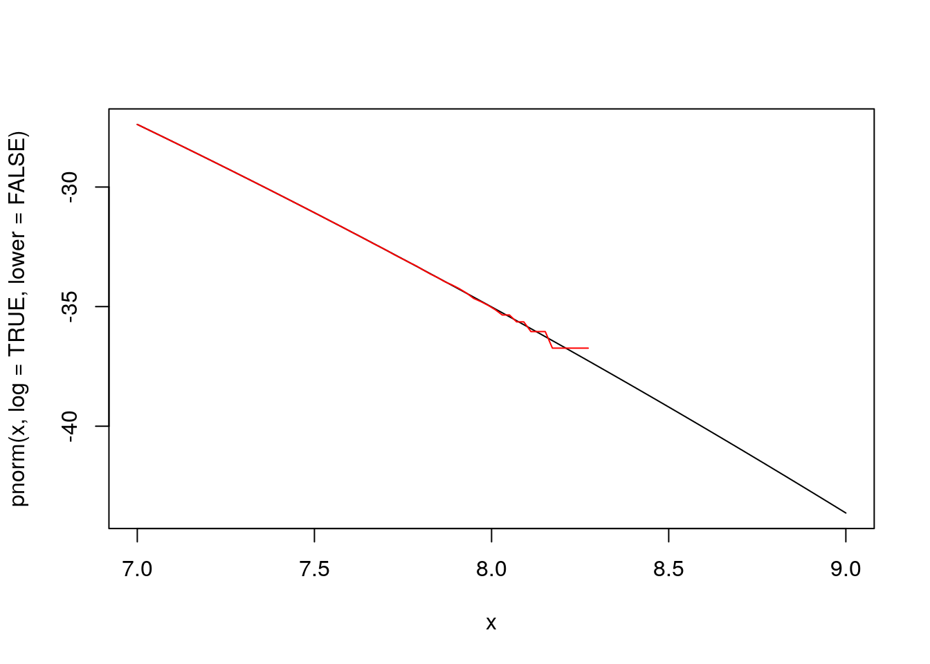
Some notes:

The problem is called catastrophic cancellation.
Floating point arithmetic is not associative or distributive.
The range considered here is quite extreme, but can be important in some cases.
The expression log(1 - pnorm(x)) produces invalid results ($-\infty$) for x above roughly 8.3.
Most R cdf functions allow lower.tail and log.p arguments (shortened to log and lower here)
The functions expm1 and log1p can also be useful. \[\begin{align*} \texttt{expm1(x)} &= e^x - 1\\ \texttt{log1p(x)} &= \log(1+x) \end{align*}\] These functions also exist in the standard C math library.

3.4.3 Another Example

Another illustration is provided by the behavior of the expression

\[\begin{equation*} e^{-2 x^2} - e^{-8 x^2} \end{equation*}\]

near the origin:

x <- seq(-1e-8, 1e-8, len = 101)
plot(x, exp(-2 * x ^ 2) - exp(-8 * x ^ 2), type = "l")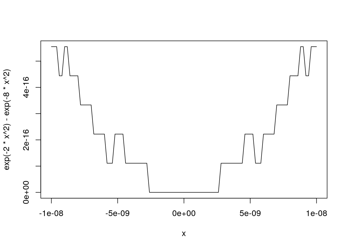

Rewriting the expression as

\[\begin{equation*} e^{-2 x^2} \left(1 - e^{-6 x^2}\right) = - e^{-2 x^2} \text{expm1}(-6 x^2) \end{equation*}\]

produces a more stable result:

plot(x, exp(-2 * x ^ 2) - exp(-8 * x ^ 2), type = "l")
lines(x, -exp(-2 * x ^ 2) * expm1(-6 * x ^ 2), col = "red")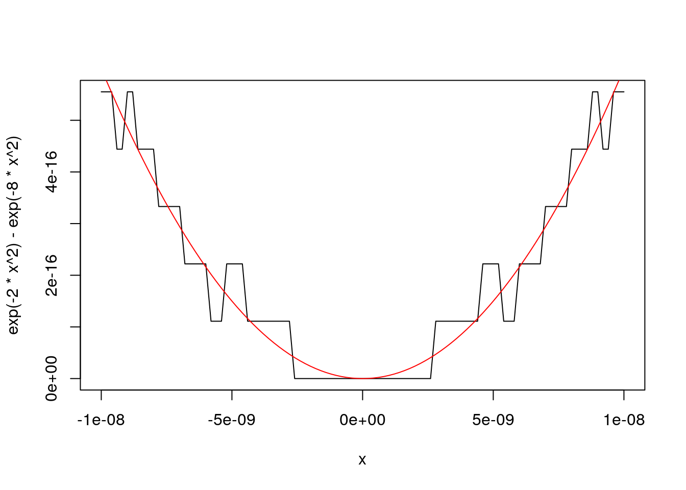

3.4.4 Sample Standard Deviations

x <- 100000000000000 + rep(c(1,2), 5)
x
##  [1] 1e+14 1e+14 1e+14 1e+14 1e+14 1e+14 1e+14 1e+14 1e+14
## [10] 1e+14
print(x, digits = 16)
##  [1] 100000000000001 100000000000002 100000000000001
##  [4] 100000000000002 100000000000001 100000000000002
##  [7] 100000000000001 100000000000002 100000000000001
## [10] 100000000000002
n <- length(x)
s <- sqrt((sum(x^2) - n * mean(x)^2) / (n - 1))
s
## [1] 0
s == 0
## [1] TRUE
y <- rep(c(1,2), 5)
y
##  [1] 1 2 1 2 1 2 1 2 1 2
sqrt((sum(y^2) - n * mean(y)^2) / (n - 1))
## [1] 0.5270463
sd(x)
## [1] 0.5270463
sd(y)
## [1] 0.5270463

The “computing formula” $\sum x_i^2 - n \overline{x}^2$ is not numerically stable. * A two-pass algorithm that first computes the mean and then computes $\sum (x_i - \overline{x})^2$ works much better. * There are also reasonably stable one-pass algorithms.

3.4.5 Truncated Normal Distribution

Sometimes it is useful to simulate from a standard normal distribution conditioned to be at least $a$, or truncated from below at $a$.

The CDF is

\[\begin{equation*} F(x|a) = \frac{\Phi(x) - \Phi(a)}{1 - \Phi(a)} \end{equation*}\]

for $x \ge a$.

The inverse CDF is

\[\begin{equation*} F^{-1}(u|a) = \Phi^{-1}(\Phi(a) + u (1 - \Phi(a))) \end{equation*}\]

This can be computed using

Finv0 <- function(u, a) {
    p <- pnorm(a)
    qnorm(p + u * (1 - p))
}

Some plots to look at:

u <- (1:100) / 101
plot(u, Finv0(u, 0), type = "l")
plot(u, Finv0(u, 2), type = "l")
plot(u, Finv0(u, 4), type = "l")
plot(u, Finv0(u, 8), type = "l")

An improved version:

Finv1 <- function(u, a) {
    q <- pnorm(a, lower.tail = FALSE)
    qnorm(q * (1 - u), lower.tail = FALSE)
}

lines(u, Finv1(u, 8), col = "red")

This could be further improved if the tails need to be more accurate.

3.5 Interger Arithmetic

Integer data types can be signed or unsigned; they have a finite range.

Almost all computers now use binary place-value for unsigned integers and two’s complement for signed integers.

Ranges are

Type	Range
unsigned:	$0,1,\dots, 2^n - 1$
signed:	$-2^{n-1}, \dots, 2^{n-1} -1$.

For C int and Fortran integer the value $n=32$ is almost universal.

If the result of +, *, or - is representable, then the operation is exact; otherwise it -overflows_.

The result of / is typically truncated; some combinations can overflow.

Typically overflow is silent.

Integer division by zero signals an error; on Linux a SIGFPE (floating point error signal!) is signaled.

It is useful to distinguish between

data that are semantically integral, like counts;
data that are stored as integers.

Semantic integers can be stored as integer or double precision floating point data

32-bit integers need 4 bytes of storage each; the range of possible values is $[-2^{31}, 2^{31} - 1]$.
Double precision floating point numbers need 8 bytes; the range of integers that can be represented exactly is $[-2^{53},2^{53}]$.
Arithmetic on integers can be faster that floating point arithmetic but this is not always true, especially if integer calculations are checked for overflow.
Storage type matters most when calling code in low level languages like C or FORTRAN.

Storing scaled floating point values as small integers (e.g. single bytes) can save space.

As data sets get larger, being able to represent integers larger than $2^{31}-1$ is becoming important.

Detecting integer overflow portably is hard; one possible strategy: use double precision floating point for calculation and check whether the result fits.

This works if integers are 32-bit and double precision is 64-bit IEEE
These assumptions are almost universally true but should be tested at compile time.

Other strategies may be faster, in particular for addition, but are harder to implement.

You can find out how R detects integer overflow by looking in the R source

https://svn.r-project.org/R/trunk/src/main/arithmetic.c

3.6 Floating Point Arithmetic

Floating point numbers are represented by a sign $s$, a significand or mantissa $sig$, and an exponent $exp$; the value of the number is

\[\begin{equation*} (-1)^s \times sig \times 2^{exp} \end{equation*}\]

The significand and the exponent are represented as binary integers.

Bases other than 2 were used in the past, but virtually all computers now follow the IEEE standard number 754 (IEEE 754 for short; the corresponding ISO standard is ISO/IEC/IEEE 60559:2011).

IEEE 754 specifies the number of bits to use:

	sign	significand	exponent	total
single precision	1	23	8	32
double precision	1	52	11	64
extended precision	1	64	15	80

A number is normalized if $1 \le sig < 2$. Since this means it looks like

\[\begin{equation*} 1.something \times 2^{exp} \end{equation*}\]

we can use all bits of the mantissa for the $something$ and get an extra bit of precision from the implicit leading one. Numbers smaller in magnitude than $1.0 \times 2^{exp_{min}}$ can be represented with reduced precision as

\[\begin{equation*} 0.something \times 2^{exp_{min}} \end{equation*}\]

These are denormalized numbers.

Denormalized numbers allow for gradual underflow. IEEE 745 includes them; many older approaches did not.

Some GPUs set denormalized numbers to zero.

For a significand with three bits, $exp_{min} = -1$, and $exp_{max} = 2$ the available nonnegative floating point numbers look like this:

Normalized numbers are blue, denormalized numbers are red.

Zero is not a normalized number (but all representations include it).

Without denormalized numbers, the gap between zero and the first positive number is larger than the gap between the first and second positive numbers.

There are actually two zeros in this framework: $+0$ and $-0$. One way to see this in R:

zp <- 0       ## this is read as +0
zn <- -1 * 0  ## or zn <- -0; this produces -0
zn == zp
## [1] TRUE
1 / zp
## [1] Inf
1 / zn
## [1] -Inf

This can identify the direction from which underflow occurred.

The IEEE 754 representation of floating point numbers looks like

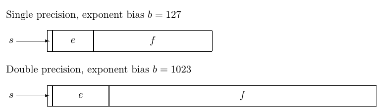
The exponent is represented by a nonnegative integer $e$ from which a bias $b$ is subtracted.

The fractional part is a nonnegative integer $f$.

The representation includes several special values: $\pm\infty$, NaN () values:

	$e$	$f$	Value
Normalized	$1 \le e \le 2b$	any	$\pm1.f\times 2^{e-b}$
Denormalized	0	$\neq 0$	$\pm0.f\times 2^{-b+1}$
Zero	0	0	$\pm 0$
Infinity	$2b+1$	0	$\pm\infty$
NaN	$2b+1$	$\neq 0$	NaN

$1.0/0.0$ will produce $+\infty$; $0.0/0.0$ will produce NaN.

On some systems a flag needs to be set so $0.0/0.0$ does not produce an error.

Library functions like $\exp$, $\log$ will behave predictably on most systems, but there are still some where they do not.

Comparisons like x <= y or x == y should produce FALSE if one of the operands is NaN; most Windows C compilers violate this.

The range of exactly representable integers in double precision: \[\begin{equation*} \pm(2^{53}-1) \approx \pm 9.0072 \times 10^{15} \end{equation*}\] The smallest positive (denormalized) double precision number: \[\begin{equation*} 2^{-b+1}\times 2^{-52} = 2^{-1074} \approx 4.940656 \times 10^{-324} \end{equation*}\]

3.7 Machine Epsilon and Machine Unit

Let $m$ be the smallest and $M$ the largest positive finite normalized floating point numbers.

Let ${\text{fl}}(x)$ be the closest floating point number to $x$.

3.7.1 Machine Unit

The is the smallest number ${\mathbf{u}}$ such that

\[ |{\text{fl}}(x) - x| \le {\mathbf{u}}\, |x| \]

for all $x \in [m, M]$; this implies that for every $x \in [m, M]$

\[ {\text{fl}}(x) = x(1+u) \]

for some $u$ with $|u| \le {\mathbf{u}}$. For double precision IEEE arithmetic,

\[ {\mathbf{u}}= \frac{1}{2} 2^{1 - 53} = 2^{-53} \approx 1.110223 \times 10^{-16} \]

3.7.2 Machine Epsilon

The ${\varepsilon_{m}}$ is the smallest number $x$ such that

\[ {\text{fl}}(1+x) \neq 1 \]

For double precision IEEE arithmetic,

\[ {\varepsilon_{m}}= 2^{-52} = 2.220446 \times 10^{-16} = 2 {\mathbf{u}}\]

${\mathbf{u}}$ and ${\varepsilon_{m}}$ are very close; they are sometimes used interchangeably.

3.7.3 Computing Machine Constants

A standard set of routines for computing machine information is provided by

Cody, W. J. (1988) MACHAR: A subroutine to dynamically determine machine parameters. Transactions on Mathematical Software, 14, 4, 303-311.

Simple code for computing machine epsilon is available.

Using R code:

eps <- 2
neweps <- eps / 2
while (1 + neweps != 1) {
    eps <- neweps
    neweps <- neweps / 2.0
}
eps
## [1] 2.220446e-16
.Machine$double.eps
## [1] 2.220446e-16
eps == .Machine$double.eps
## [1] TRUE

Analogous C code compiled with

cc -Wall -pedantic -o eps eps.c

produces

luke@itasca2 macheps% ./eps
epsilon = 2.22045e-16

The same C code compiled with optimization (and an older gcc compiler) on a i386 system

cc -Wall -pedantic -o epsO2 eps.c -O2

produced

luke@itasca2 macheps% ./epsO2
epsilon = 1.0842e-19

Why does this happen?

Here is a hint:

log2(.Machine$double.eps)
## [1] -52
log2(1.0842e-19)
## [1] -63

3.7.4 Some Notes

Use equality tests x == y for floating point numbers with caution

Multiplies can overflow—use logs (log likelihoods)

Cases where care is needed:
survival likelihoods
mixture likelihoods.

Double precision helps a lot.

3.8 Machine Characteristics in R

The variable .Machine contains values for the characteristics of the current machine:

.Machine
## $double.eps
## [1] 2.220446e-16
## 
## $double.neg.eps
## [1] 1.110223e-16
## 
## $double.xmin
## [1] 2.225074e-308
## 
## $double.xmax
## [1] 1.797693e+308
## 
## $double.base
## [1] 2
## 
## $double.digits
## [1] 53
## 
## $double.rounding
## [1] 5
## 
## $double.guard
## [1] 0
## 
## $double.ulp.digits
## [1] -52
## 
## $double.neg.ulp.digits
## [1] -53
## 
## $double.exponent
## [1] 11
## 
## $double.min.exp
## [1] -1022
## 
## $double.max.exp
## [1] 1024
## 
## $integer.max
## [1] 2147483647
## 
## $sizeof.long
## [1] 8
## 
## $sizeof.longlong
## [1] 8
## 
## $sizeof.longdouble
## [1] 16
## 
## $sizeof.pointer
## [1] 8

The help page gives details.

3.9 Floating Point Equality

R FAQ 7.31: Why doesn’t R think these numbers are equal?

b <- 1 - 0.8
b
## [1] 0.2
b == 0.2
## [1] FALSE
b - 0.2
## [1] -5.551115e-17

Answer from FAQ:

The only numbers that can be represented exactly in R’s numeric type are integers and fractions whose denominator is a power of 2. Other numbers have to be rounded to (typically) 53 binary digits accuracy. As a result, two floating point numbers will not reliably be equal unless they have been computed by the same algorithm, and not always even then. For example
a <- sqrt(2)
a * a == 2
## [1] FALSE
a * a - 2
## [1] 4.440892e-16
The function all.equal() compares two objects using a numeric tolerance of .Machine$double.eps ^ 0.5. If you want much greater accuracy than this you will need to consider error propagation carefully.

The function all.equal() returns either TRUE or a string describing the failure. To use it in code you would use something like

if (identical(all.equal(x, y), TRUE)) ...
else ...

but using an explicit tolerance test is probably clearer.

Bottom line: be VERY CAREFUL about using equality comparisons with floating point numbers.

3.10 Reference

David Goldberg (1991). What Every Computer Scientist Should Know About Floating-Point Arithmetic, ACM Computing Surveys. Edited version available on line.

	\(e\)	\(f\)	Value
Normalized	\(1 \le e \le 2b\)	any	\(\pm1.f\times 2^{e-b}\)
Denormalized	0	\(\neq 0\)	\(\pm0.f\times 2^{-b+1}\)
Zero	0	0	\(\pm 0\)
Infinity	\(2b+1\)	0	\(\pm\infty\)
NaN	\(2b+1\)	\(\neq 0\)	NaN

Type	Range
unsigned:	\(0,1,\dots, 2^n - 1\)
signed:	\(-2^{n-1}, \dots, 2^{n-1} -1\).