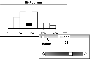
Figure 18: Slider-controlled animation of a histogram.
In Section 6.6 we used a loop to control a dynamic simulation in which points in a histogram of one variable were selected and deselected in the order of a second variable. Let's look at how to run the same simulation using a slider to control the simulation.
A slider is a modeless dialog box containing a scroll bar and a value display field. As the scroll bar is moved the displayed value is changed and an action is taken. The action is defined by an action function given to the scroll bar, a function that is called with one value, the current slider value, each time the value is changed by the user. There are two kinds of sliders, sequence sliders and interval sliders. Sequence sliders take a sequence (a list or a vector) and scroll up and down the sequence. The displayed value is either the current sequence element or the corresponding element of a display sequence. An interval slider dialog takes an interval, divides it into a grid and scrolls through the grid. By default a grid of around 30 points is used; the exact number and the interval end points are adjusted to give nice printed values. The current interval point is displayed in the display field.
For our example let's use a sequence slider to scroll through the elements of the hardness list in order and select the corresponding element of abrasion-loss. The expression
(def h (histogram abrasion-loss))sets up a histogram and saves its plot object in the variable h. The function sequence-slider-dialog takes a list or vector and opens a sequence slider to scroll through its argument. To do something useful with this dialog we need to give it an action function as the value of the keyword argument :action. The function should take one argument, the current value of the sequence controlled by the slider. The expression
(sequence-slider-dialog (order hardness) :action
                        #'(lambda (i)
                            (send h :unselect-all-points)
                            (send h :point-selected i t)))
sets up a slider for moving the selected point in the abrasion-loss
histogram along the order of the hardness variable. The histogram
and scroll bar are shown in Figure 18.

Figure 18: Slider-controlled animation of a histogram.
The action function is called every time the slider is moved. It is called with the current element of the sequence (order hardness), the index of the point to select. It clears all current selections and then selects the point specified in the call from the slider. The body of the function is almost identical to the body of the dotimes loop used in Section 6.6. The slider is thus an interactive, graphically controlled version of this loop.
As another example, suppose we would like to examine the effect of changing the exponent in a Box-Cox power transformation

on a probability plot. As a first step we might define a function to compute the power transformation and normalize the result to fall between zero and one:
(defun bc (x p)
  (let* ((bcx (if (< (abs p) .0001) (log x) (/ (^ x p) p)))
         (min (min bcx))
         (max (max bcx)))
    (/ (- bcx min) (- max min))))
This definition uses the let* form to establish
some local variable bindings. The let* form is like the
let form used above except that let* defines its
variables sequentially, allowing a variable to be defined in terms of
other variables already defined in the let* expression;
let on the other hand creates its assignments in parallel. In
this case the variables min and max are defined in
terms of the variable bcx.
Next we need a set of positive numbers to transform. Let's use a
sample of thirty observations from a  distribution and
order the observations:
(def x (sort-data (chisq-rand 30 4)))
The normal quantiles of the expected uniform order statistics are given by
(def r (normal-quant (/ (iseq 1 30) 31)))and a probability plot of the untransformed data is constructed using
(def myplot (plot-points r (bc x 1)))Since the power used is 1 the function bc just rescales the data.
There are several ways to set up a slider dialog to control the power parameter. The simplest approach is to use the function interval-slider-dialog:
(interval-slider-dialog (list -1 2)
                        :points 20
                        :action #'(lambda (p)
                                   (send myplot :clear nil)
                                   (send myplot :add-points r (bc x p))))
interval-slider-dialog takes a list of two numbers, the lower and
upper bounds of an interval. The action function is called with the
current position in the interval.
This approach works fine on a Mac II but may be a bit slow on a Mac Plus or a Mac SE. An alternative is to pre-compute the transformations for a list of powers and then use the pre-computed values in the display. For example, using the powers defined in
(def powers (rseq -1 2 16))we can compute the transformed data for each power and save the result as the variable xlist:
(def xlist (mapcar #'(lambda (p) (bc x p)) powers))The function mapcar is one of several mapping functions available in Lisp. The first argument to mapcar is a function. The second argument is a list. mapcar takes the function, applies it to each element of the list and returns the list of the results
(sequence-slider-dialog xlist
                        :display powers
                        :action #'(lambda (x)
                                   (send myplot :clear nil)
                                   (send myplot :add-points r x)))
Note that we are scrolling through a list of lists and the element passed
to the action function is thus the list of current transformed values. We
would not want to see these values in the display field on the slider, so
I have used the keyword argument :display to specify an alternative
display sequence, the powers used in the transformation.