Regression models have been implemented using XLISP-STAT's object and message sending facilities. These were introduced above in Section 6.5. You might want to review that section briefly before reading on.
Let's fit a simple regression model to the bicycle data of Section 6.5. The dependent variable is separation and the independent variable is travel-space. To form a regression model use the regression-model function:
> (regression-model travel-space separation)

Least Squares Estimates:

Constant               -2.182472   (1.056688)
Variable 0             0.6603419   (0.06747931)

R Squared:              0.922901
Sigma hat:             0.5821083
Number of cases:              10
Degrees of freedom:            8

#<Object: 1966006, prototype = REGRESSION-MODEL-PROTO>
>
The basic syntax for the regression-model function is
(regression-model x y)For a simple regression x can be a single list or vector. For a multiple regression x can be a list of lists or vectors or a matrix. The regression-model function also takes several optional keyword arguments. The most important ones are :intercept, :print, and :weights. Both :intercept and :print are T by default. To get a model without an intercept use the expression
(regression-model x y :intercept nil)To form a weighted regression model use the expression
(regression-model x y :weights w)where w is a list or vector of weights the same length as y. In a weighted model the variances of the errors are assumed to be inversely proportional to the weights w.
The regression-model function prints a very simple summary of the
fit model and returns a model object as its result. To be able to examine
the model further assign the returned model object to a variable using
an expression like
![]()
(def bikes (regression-model travel-space separation :print nil))I have given the keyword argument :print nil to suppress the printing of the summary, since we have already seen it. To find out what messages are available use the :help message:
> (send bikes :help)
REGRESSION-MODEL-PROTO
Normal Linear Regression Model
Help is available on the following:

:ADD-METHOD :ADD-SLOT :BASIS :CASE-LABELS :COEF-ESTIMATES :COEF-STANDARD-ERRORS
:COMPUTE :COOKS-DISTANCES :DELETE-METHOD :DELETE-SLOT :DF :DISPLAY :DOC-TOPICS
:DOCUMENTATION :EXTERNALLY-STUDENTIZED-RESIDUALS :FIT-VALUES :GET-METHOD
:HAS-METHOD :HAS-SLOT :HELP :INCLUDED :INTERCEPT :INTERNAL-DOC :ISNEW
:LEVERAGES :METHOD-SELECTORS :NEW :NUM-CASES :NUM-COEFS :NUM-INCLUDED
:OWN-METHODS :OWN-SLOTS :PARENTS :PLOT-BAYES-RESIDUALS :PLOT-RESIDUALS
:PRECEDENCE-LIST :PREDICTOR-NAMES :PRINT :R-SQUARED :RAW-RESIDUALS
:RESIDUAL-SUM-OF-SQUARES :RESIDUALS :RESPONSE-NAME :RETYPE :SAVE :SHOW
:SIGMA-HAT :SLOT-NAMES :SLOT-VALUE :STUDENTIZED-RESIDUALS :SUM-OF-SQUARES
:SWEEP-MATRIX :TOTAL-SUM-OF-SQUARES :WEIGHTS :X :X-MATRIX :XTXINV :Y PROTO
NIL
>
Many of these messages are self explanatory, and many have already been used by the :display message, which regression-model sends to the new model to print the summary. As examples let's try the :coef-estimates and :coef-standard-errors messages
> (send bikes :coef-estimates)
(-2.182472 0.6603419)
> (send bikes :coef-standard-errors)
(1.056688 0.06747931)
>
The :plot-residuals message will produce a residual plot . To find out what residuals are plotted against let's look at the help information:
> (send bikes :help :plot-residuals)
:PLOT-RESIDUALS

Message args: (&optional x-values)
Opens a window with a plot of the residuals. If X-VALUES are not supplied
the fitted values are used. The plot can be linked to other plots with the
link-views function. Returns a plot object.
NIL
>
Using the expressions
        (plot-points travel-space separation)
        (send bikes :plot-residuals travel-space)
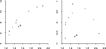
Figure 15: Linked raw data and residual plots for the bicycles
example.
we can construct two plots of the data as shown in Figure 15. By linking the plots we can use the mouse to identify points in both plots simultaneously. A point that stands out is observation 6 (starting the count at 0, as usual).
The plots both suggest that there is some curvature in the data; this curvature is particularly pronounced in the residual plot if you ignore observation 6 for the moment. To allow for this curvature we might try to fit a model with a quadratic term in travel-space:
> (def bikes2  (regression-model (list travel-space (^ travel-space 2))
                                 separation))

Least Squares Estimates:

Constant               -16.41924   (7.848271)
Variable 0              2.432667   (0.9719628)
Variable 1           -0.05339121   (0.02922567)

R Squared:             0.9477923
Sigma hat:             0.5120859
Number of cases:              10
Degrees of freedom:            7

BIKES2
>
I have used the exponentiation function ``^'' to compute the
square of travel-space. Since I am now forming a multiple
regression model the first argument to
regression-model is a list of the x variables.
You can proceed in many directions from this point. If you want to calculate Cook's distances for the observations you can first compute internally studentized residuals as
(def studres (/ (send bikes2 :residuals)
                (* (send bikes2 :sigma-hat)
                   (sqrt (- 1 (send bikes2 :leverages))))))
Then Cook's distances are obtained as
> (* (^ studres 2)
     (/ (send bikes2 :leverages) (- 1 (send bikes2 :leverages)) 3))
(0.166673 0.00918596 0.03026801 0.01109897 0.009584418 0.1206654 0.581929
0.0460179 0.006404474 0.09400811)
The seventh entry -- observation 6, counting from zero -- clearly
stands out.
Another approach to examining residuals for possible outliers is to use the Bayesian residual plot proposed by Chaloner and Brant [7], which can be obtained using the message :plot-bayes-residuals . The expression (send bikes2 :plot-bayes-residuals) produces the plot in Figure 16.
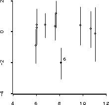
Figure 16: Bayes residual plot for bicycle data.
The bars represent mean  of the posterior distribution of the
actual realized errors, based on an improper uniform prior distribution on
the regression coefficients. The y axis is in units of
of the posterior distribution of the
actual realized errors, based on an improper uniform prior distribution on
the regression coefficients. The y axis is in units of  .
Thus this plot suggests the probability that point 6 is three or more
standard deviations from the mean is about 3%; the probability that it is
at least two standard deviations from the mean is around 50%.
.
Thus this plot suggests the probability that point 6 is three or more
standard deviations from the mean is about 3%; the probability that it is
at least two standard deviations from the mean is around 50%.
Several other methods are available for residual and case analysis. These include :studentized-residuals and :cooks-distances, which we could have used above instead of calculating these quantities from their definitions. Another useful message is :included, which can be used to change the cases to be used in estimating a model. Further details on these messages are available in their help information.