After producing a scatterplot of a data set we might like to add a line, a regression line for example, to the plot. As an example, Devore and Peck [11, page 105, Example 2,] describe a data set collected to examine the effect of bicycle lanes on drivers and bicyclists. The variables given by
(def travel-space (list 12.8 12.9 12.9 13.6 14.5 14.6 15.1 17.5 19.5 20.8))
(def separation (list 5.5 6.2 6.3 7.0 7.8 8.3 7.1 10.0 10.8 11.0))
represent the distance between the cyclist and the roadway center line and the distance between the cyclist and a passing car, respectively, recorded in ten cases. A regression line fit to these data, with separation as the dependent variable, has a slope of 0.66 and an intercept of -2.18. Let's see how to add this line to a scatterplot of the data.
We can use the expression
(plot-points travel-space separation)to produce a scatterplot of these points. To be able to add a line to the plot, however, we must be able to refer to it within XLISP-STAT. To accomplish this let's assign the result returned by the plot-points function to a symbol
(def myplot (plot-points travel-space separation))The result returned by plot-points is an XLISP-STAT object . To use an object you have to send it messages. This is done using the send function, as in the expression
(send object message argument1 ... )I will use the expression
(send myplot :abline -2.18 0.66)to tell myplot to add the graph of a line a + b x, with
 and
and  , to itself. The message selector is
:abline, the numbers -2.18 and
0.66 are the arguments. The message consists of the selector
and the arguments. Message selectors are always Lisp keywords; that is,
they are symbols that start with a colon. Before typing in this
expression you might want to resize and rearrange the listener window
so you can see the plot and type commands at the same time. Once you
have resized the listener window you can easily switch between the
small window and a full size window by clicking in the zoom box at the
right corner of the window title bar. The resulting plot is shown
in Figure 13
, to itself. The message selector is
:abline, the numbers -2.18 and
0.66 are the arguments. The message consists of the selector
and the arguments. Message selectors are always Lisp keywords; that is,
they are symbols that start with a colon. Before typing in this
expression you might want to resize and rearrange the listener window
so you can see the plot and type commands at the same time. Once you
have resized the listener window you can easily switch between the
small window and a full size window by clicking in the zoom box at the
right corner of the window title bar. The resulting plot is shown
in Figure 13
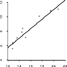
Figure 13: Scatterplot of bicycle data with fitted line.
Scatter plot objects understand a number of other messages. One other
message is the :help message
![]() :
:
> (send myplot :help)
> (send scatterplot-proto :help)
SCATTERPLOT-PROTO
Scatterplot.
Help is available on the following:

:ABLINE :ACTIVATE :ADD-FUNCTION :ADD-LINES :ADD-METHOD :ADD-MOUSE-MODE
:ADD-POINTS :ADD-SLOT :ADD-STRINGS :ADJUST-HILITE-STATE
:ADJUST-POINT-SCREEN-STATES :ADJUST-POINTS-IN-RECT :ADJUST-TO-DATA
:ALL-POINTS-SHOWING-P :ALL-POINTS-UNMASKED-P :ALLOCATE
:ANY-POINTS-SELECTED-P :APPLY-TRANSFORMATION :BACK-COLOR :BRUSH
:BUFFER-TO-SCREEN :CANVAS-HEIGHT :CANVAS-WIDTH :CLEAR :CLEAR-LINES
:CLEAR-MASKS :CLEAR-POINTS :CLEAR-STRINGS ....
The list of topics will be the same for all scatter plots but will be somewhat different for rotating plots, scatterplot matrices or histograms.
The :clear message, as its name suggests, clears the plot and allows you to build up a new plot from scratch. Two other useful messages are :add-points and :add-lines. To find out how to use them we can use the :help message with :add-points or :add-lines as arguments:
> (send myplot :help :add-points)
:ADD-POINTS
Method args: (points &key point-labels (draw t))
Adds points to plot. POINTS is a list of sequences, POINT-LABELS a list of
strings. If DRAW is true the new points are added to the screen.
NIL
> (send myplot :help :add-lines)
:ADD-LINES
Method args: (lines &key type (draw t))
Adds lines to plot. LINES is a list of sequences, the coordinates of the line
starts. TYPE is normal or dashed. If DRAW is true the new lines are added to the
screen.
NIL
>
The plot produced above shows some curvature in the data. A regression of separation on a linear and a quadratic term in travel-space produces estimates of -16.41924 for the constant, 2.432667 as the coefficient of the linear term and -0.05339121 as the coefficient of the quadratic term. Let's use the :clear, :add-points and :add-lines messages to change myplot to show the data along with the fitted quadratic model. First we use the expressions
(def x (rseq 12 22 50))
(def y (+ -16.41924 (* 2.432667 x) (* -0.05339121 (* x x))))
to define x as a grid of 50 equally spaced points between 12 and 22 and y as the fitted response at these x values. Then the expressions
(send myplot :clear)
(send myplot :add-points travel-space separation)
(send myplot :add-lines x y)
change myplot to look like Figure 14.
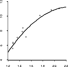
Figure 14: Scatterplot of bicycle data with fitted curve.
Of course we could have used plot-points to get a new plot and just modified that plot with :add-lines, but the approach used here allowed us to try out all three messages.