Chapter 8 Statistical Learning

8.1 Some Machine Learning Terminology

Two forms of learning:

• supervised learning: features and responses are available for a training set, and a way of predicting response from features of new data is to be learned.

• unsupervised learning: no distinguished responses are available; the goal is to discover patterns and associations among features.

Classification and regression are supervised learning methods.

Clustering, multi-dimensional scaling, and principal curves are unsupervised learning methods.

Data mining involves extracting information from large (many cases and/or many variables), messy (many missing values, many different kinds of variables and measurement scales) data bases.

Machine learning often emphasizes methods that are sufficiently fast and automated for use in data mining.

Machine learning is now often considered a branch of Artificial Intelligence (AI).

Tree models are popular in machine learning

• supervised: as predictors in classification and regression settings

• unsupervised: for describing clustering results.

Some other methods often associated with machine learning:

• Bagging

• Boosting

• Random Forests

• Support Vector Machines

• Neural Networks

References:

T. Hastie, R. Tibshirani, and J. Friedman (2009). The Elements of Statistical Learning, 2nd Ed..

G. James, D. Witten, T. Hastie, and R. Tibshirani (2021). An Introduction to Statistical Learning, with Applications in R, 2nd Ed..

D. Hand, H, Mannila, and P. Smyth (2001). Principles of Data Mining.

C. M. Bishop (2006). Pattern Recognition and Machine Learning.

M. Shu (2008). Kernels and ensembles: perspectives on statistical learning, The American Statistician 62(2), 97–109.

Some examples are available on line on line.

8.2 Tree Models

Tree models were popularized by a book and software named CART, for Classification and Regression Trees.

The name CART was trademarked and could not be used by other implementations.

Tree models partition the predictor space based on a series of binary splits.

Leaf nodes predict a response:

• a category for classification trees;

• a numerical value for regression trees.

Regression trees may also use a simple linear model within leaf nodes of the partition.

Using rpart a tree model for predicting union membership can be constructed by

data(trade.union, package = "SemiPar")
library(rpart)
trade.union$member.fac <-
    as.factor(ifelse(trade.union$union.member,
                     "yes",
                     "no"))
fit <- rpart(member.fac ~ wage + age + years.educ,
             data = trade.union)
plot(fit)
text(fit, use.n = TRUE)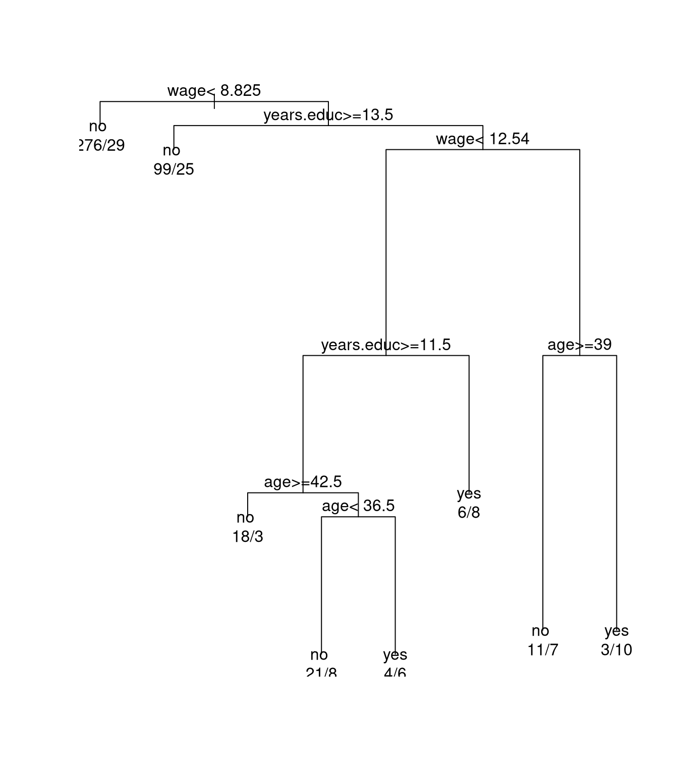

Regression trees use a constant fit by default.

A regression tree for the California air pollution data:

data(calif.air.poll, package = "SemiPar")
library(rpart)
fit2 <-
    rpart(ozone.level ~ daggett.pressure.gradient +
              inversion.base.height +
              inversion.base.temp,
          data = calif.air.poll)
plot(fit2)
text(fit2)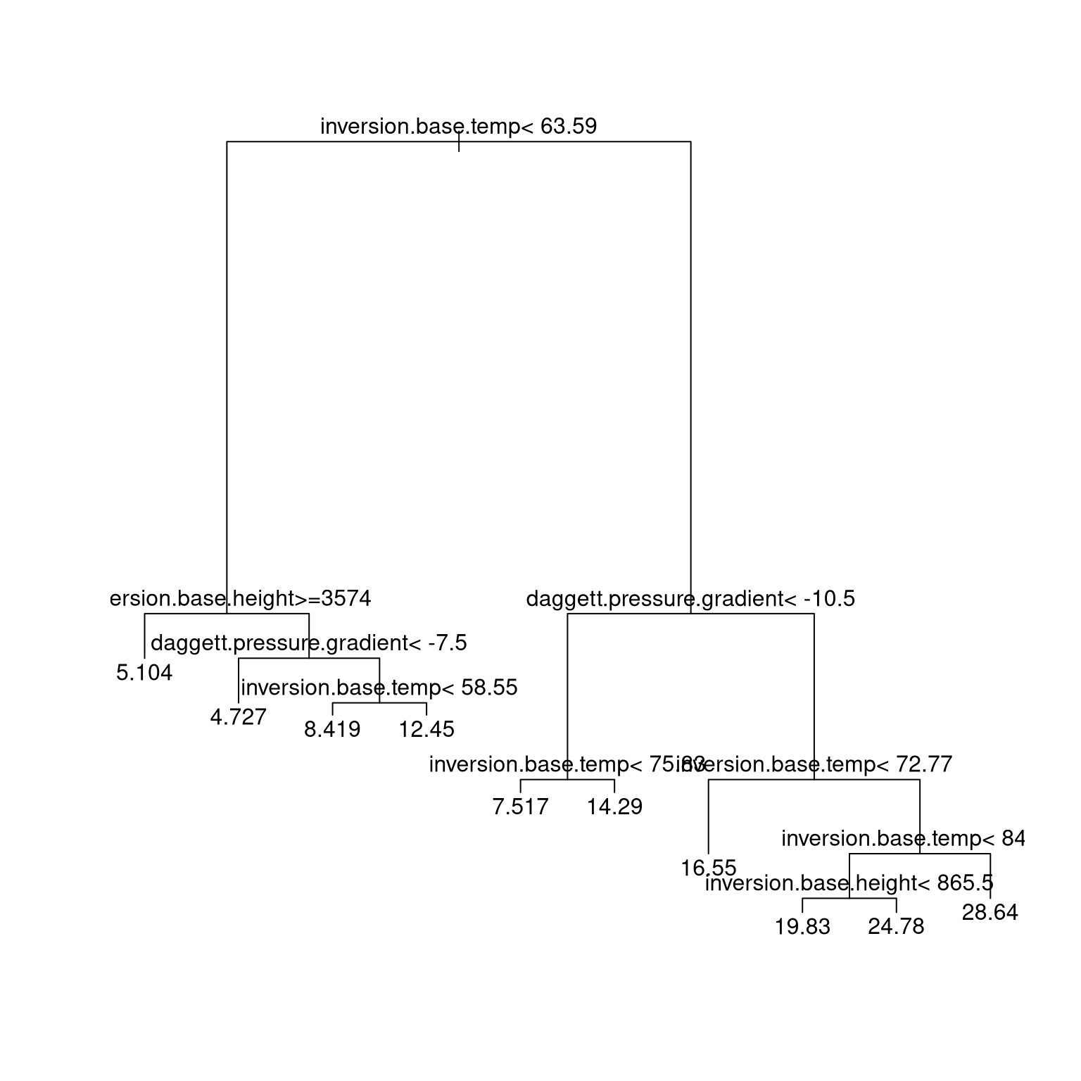

Tree models are flexible but simple; results are easy to explain to non-specialists.

Small changes in data

• can change tree structure substantially;

• usually do not change predictive performance much.

Fitting procedures usually consist of two phases:

• growing a large tree;

• pruning back the tree to reduce over-fitting.

Tree growing usually uses a greedy approach. Pruning usually minimizes a penalized goodness of fit measure

\[\begin{equation*} R(\mathcal{T}) + \lambda \text{size}(\mathcal{T}) \end{equation*}\]

with \(R\) a raw measure of goodness of fit.

The parameter \(\lambda\) can be chosen by some form of cross-validation.

For regression trees, mean square prediction error is usually used for both growing and pruning.

For classification trees

• growing usually uses a loss function that rewards class purity, e.g. a Gini index \[G_m = \sum_{k=1}^K \widehat{p}_{mk}(1 - \widehat{p}_{mk})\] or a cross-entropy \[D_m = - \sum_{k=1}^K \widehat{p}_{mk}\log \widehat{p}_{mk}\] with \(\widehat{p}_{mk}\) the proportion of training observations in region \(m\) that are in class \(k\).

• Pruning usually focuses on minimizing classification error rates.

The rpart package provides one implementation; the tree and party packages are also available, among others.

8.3 Bagging, Boosting, and Random Forests

All three are ensemble methods: They combine weaker predictors, or learners, to form a stronger one.

A related idea is Bayesian Model Averaging (BMA).

8.3.1 Bagging: Bootstrap AGGregation

Bootstrapping in prediction models produces a sample of predictors

\[\begin{equation*} T_1^*(x),\dots,T_R^*(x). \end{equation*}\]

Usually bootstrapping is viewed as a way of assessing the variability of the predictor \(T(x)\) based on the original sample.

For predictors that are not linear in the data an aggregated estimator such as

\[\begin{equation*} T_\text{BAG}(x) = \frac{1}{R}\sum_{i=1}^R T_i^*(x) \end{equation*}\]

may be an improvement.

Other aggregations are possible; for classification trees two options are

• averaging probabilities;
• majority vote.

Bagging can be particularly effective for tree models.

Less pruning, or even no pruning, is needed since variance is reduced by averaging.

Each bootstrap sample will use about 2/3 of the observations; about 1/3 will be out of bag, or OOB. The OOB observations can be used to construct an error estimate.

For tree methods:

• The resulting predictors are more accurate than simple trees, but lose the simple interpretability.

• The total reduction in RSS or the Gini index due to splits on a particular variable can be used as a measure of variable importance.

Bumping (Bootstrap umbrella of model parameters) is another approach:

• Given a bootstrap sample of predictors \(T_1^*(x),\dots,T_R^*(x)\) choose the one that best fits the original data.

• The original sample is included in the bootstrap sample so the original predictor can be chosen if it is best.

8.3.2 Random Forests

Introduced by Breiman (2001).

Also covered by a trademark.

Similar to bagging for regression or classification trees.

Draws \(n_\text{tree}\) bootstrap samples. For each sample a tree is grown without pruning.

• At each node \(m_\text{try}\) out of \(p\) available predictors are sampled at random.

• A common choice is \(m_\text{try} \approx \sqrt{p}\).

• The best split among the sampled predictors is used.

Form an ensemble predictor by aggregating the trees.

Error rates are measured by

• at each bootstrap iteration predict data not in the sample (out-of-bag, OOB, data);

• combine the OOB error measures across samples.

Bagging without pruning for tree models is equivalent to a random forest with \(m_\text{try} = p\).

A motivation is to reduce correlation among the bootstrap trees and so increase the benefit of averaging.

The R package randomForest provides an interface to FORTRAN code of Breiman and Cutler.

The software provides measures of

• “importance” of each predictor variable;

• similarity of observations.

Some details are available in A. Liaw and M. Wiener (2002). “Classification and Regression by randomForest,” R News.

Other packages implementing random forests are a available as well.

A recent addition is the ranger package.

8.4 Boosting

Boosting is a way of improving on a weak supervised learner.

The basic learner needs to be able to work with weighted data.

The simplest version applies to binary classification with responses \(y_i = \pm 1\).

A binary classifier produced from a set of weighted training data is a function

\[\begin{equation*} G(x): \mathcal{X} \to \{-1,+1\} \end{equation*}\]

The AdaBoost.M1 (adaptive boosting) algorithm:

1. Initialize observation weights \(w_i = 1/n, i = 1,\dots,n\).
2. For \(m = 1, \dots, M\) do

1. Fit a classifier \(G_m(x)\) to the training data with weights \(w_i\).

2. Compute the weighted error rate \[\begin{equation*} \text{err}_m = \frac{\sum_{i=1}^n w_i 1_{\{y_i \neq G_m(x_i)\}}}{\sum_{i=1}^n w_i}. \end{equation*}\]

3. Compute \(\alpha_m = \log((1 - \text{err}_m) / \text{err}_m)\).

4. Set \(w_i \leftarrow w_i \exp(\alpha_m 1_{\{y_i \neq G_m(x_i)\}})\)

3. Output \(G(x) = \text{sign}\left(\sum_{i=1}^M \alpha_m G_m(x)\right)\)

The weights are adjusted to put more weight on points that were classified incorrectly.

These ideas extend to multiple categories and to continuous responses.

Empirical evidence suggests boosting is successful in a range of problems.

Theoretical investigations support this.

The resulting classifiers are closely related to additive models constructed from a set of elementary basis functions.

The number of steps \(M\) plays the role of a model selection parameter

• too small a value produces a poor fit

• too large a value fits the training data too well

Some form of regularization, e.g. based on a validation sample, is needed.

Other forms of regularization, e.g. variants of shrinkage, are possible as well.

A variant for boosting regression trees:

1. Set \(\widehat{f}(x) = 0\) and \(r_i = y_i\) for all \(i\) in the training set.
2. For \(m = 1, \dots, M\):

1. Fit a tree \(\widehat{f}^m(x)\) with \(d\) splits to the training data \(X, r\).

2. Update \(\widehat{f}\) by adding a shrunken version of \(\widehat{f}^m(x)\), \[\widehat{f}(x) \leftarrow \widehat{f}(x) + \lambda \widehat{f}^m(x).\]

3. Update the residuals \[r_i \leftarrow r_i - \lambda \widehat{f}^m(x)\]

3. Return the boosted model \[\widehat{f}(x) = \sum_{m = 1}^{M} \lambda \widehat{f}^m(x)\]

Using a fairly small \(d\) often works well.

With \(d = 1\) this fits an additive model.

Small values of \(\lambda\), e.g. 0.01 or 0.001, often work well.

\(M\) is generally chosen by cross-validation.

8.4.1 References on Boosting

P. Buehlmann and T. Hothorn (2007). “Boosting algorithms: regularization, prediction and model fitting (with discussion),” Statistical Science, 22(4),477–522.

Andreas Mayr, Harald Binder, Olaf Gefeller, Matthias Schmid (2014). “The evolution of boosting algorithms - from machine learning to statistical modelling,” Methods of Information in Medicine 53(6), arXiv:1403.1452.

Tianqi Chen and Carlos Guestrin (2016). XGBoost: A Scalable Tree Boosting System. In 22nd SIGKDD Conference on Knowledge Discovery and Data Mining, arXiv:1603.02754.

8.4.2 California Air Pollution Data

Load data and split out a training sample:

data(calif.air.poll, package = "SemiPar")
library(mgcv)
train <- sample(nrow(calif.air.poll), nrow(calif.air.poll) / 2)

Fit the additive linear model to the training data and compute the mean square prediction error for the test data:

fit <- gam(ozone.level ~ s(daggett.pressure.gradient)
                       + s(inversion.base.height)
                       + s(inversion.base.temp),
           data=calif.air.poll[train,])
(gam.mse <- mean((calif.air.poll$ozone.level[-train] -
                  predict(fit, calif.air.poll[-train,]))^2))
## [1] 19.52757

Fit a tree to the training data using all pedictors:

library(rpart)
tree.ca <- rpart(ozone.level ~ .,
                 data = calif.air.poll[train,])
(tree.mse <-
     mean((calif.air.poll$ozone.level[-train] -
           predict(tree.ca, calif.air.poll[-train,]))^2))
## [1] 23.40834

Use bagging on the training set:

library(randomForest)
bag.ca <- randomForest(ozone.level ~ .,
                       data = calif.air.poll[train,],
                       mtry = ncol(calif.air.poll) - 1)
(bag.mse <-
     mean((calif.air.poll$ozone.level[-train] -
           predict(bag.ca, calif.air.poll[-train,]))^2))
## [1] 21.31767

Fit a random forest:

rf.ca <- randomForest(ozone.level ~ .,
                      data = calif.air.poll[train,])
(rf.mse <- mean((calif.air.poll$ozone.level[-train] -
                predict(rf.ca, calif.air.poll[-train,]))^2))
## [1] 20.87033

Use gbm from the gbm package to fit boosted regression trees:

library(gbm)
boost.ca <- gbm(ozone.level ~ ., data = calif.air.poll[train,],
                n.trees = 100)
## Distribution not specified, assuming gaussian ...
(gbm1.mse <- mean((calif.air.poll$ozone.level[-train] -
                   predict(boost.ca, calif.air.poll[-train,],
                           n.trees = 100))^2))
## [1] 21.46409
boost.ca2 <- gbm(ozone.level ~ ., data = calif.air.poll[train,],
                 n.trees = 100, interaction.depth=2)
## Distribution not specified, assuming gaussian ...
(gbm2.mse <- mean((calif.air.poll$ozone.level[-train] -
                   predict(boost.ca2, calif.air.poll[-train,],
                           n.trees = 100))^2))
## [1] 20.73196

Results:

Method	MSE
gam	19.53
tree	23.41
bagged	21.32
randomForest	20.87
boosted	21.46	\(M = 100\)
	20.73	\(M = 100, d = 2\)

These results were obtained without first re-scaling the predictors.

Some examples are available on line on line.

8.5 Support Vector Machines

Support vector machines are a method of classification.

The simplest form is for binary classification with training data \((x_1,y_1),\dots,(x_n,y_n)\) with

\[\begin{align*} \renewcommand{\mathbb{R}}{\mathbb{R}} x_i &\in \mathbb{R}^p\\ y_i &\in \{-1,+1\} \end{align*}\]

Various extensions to multiple classes are available; one uses a form of majority vote among all pairwise classifiers.

Extensions to continuous resposes are also available.

An R implementation is svm in package e1071.

8.5.1 Support Vector Classifiers

A linear binary classifier is of the form

\[\begin{equation*} G(x) = \text{sign}(x^T\beta + \beta_0) \end{equation*}\]

One way to choose a classifier is to minimize a penalized measure of misclassification

\[\begin{equation*} \renewcommand{\Norm}[1]{\|{#1}\|} \min_{\beta,\beta_0} \sum_{i=1}^n(1 - y_i f(x))_+ + \lambda \|{\beta}\|^2 \end{equation*}\]

with \(f(x) = x^T\beta + \beta_0\).

• The misclassification cost is zero for correctly classified points far from the bundary

• The cost increases for misclassified points farther from the boundary.

The misclassification cost is qualitatively similar to the negative log-likelihood for a logistic regression model,

\[ \rho(y_i, f(x)) = - y_i f(x) + \log\left(1 + e^{y_i f(x)}\right) = \log\left(1 + e^{-y_i f(x)}\right) \]

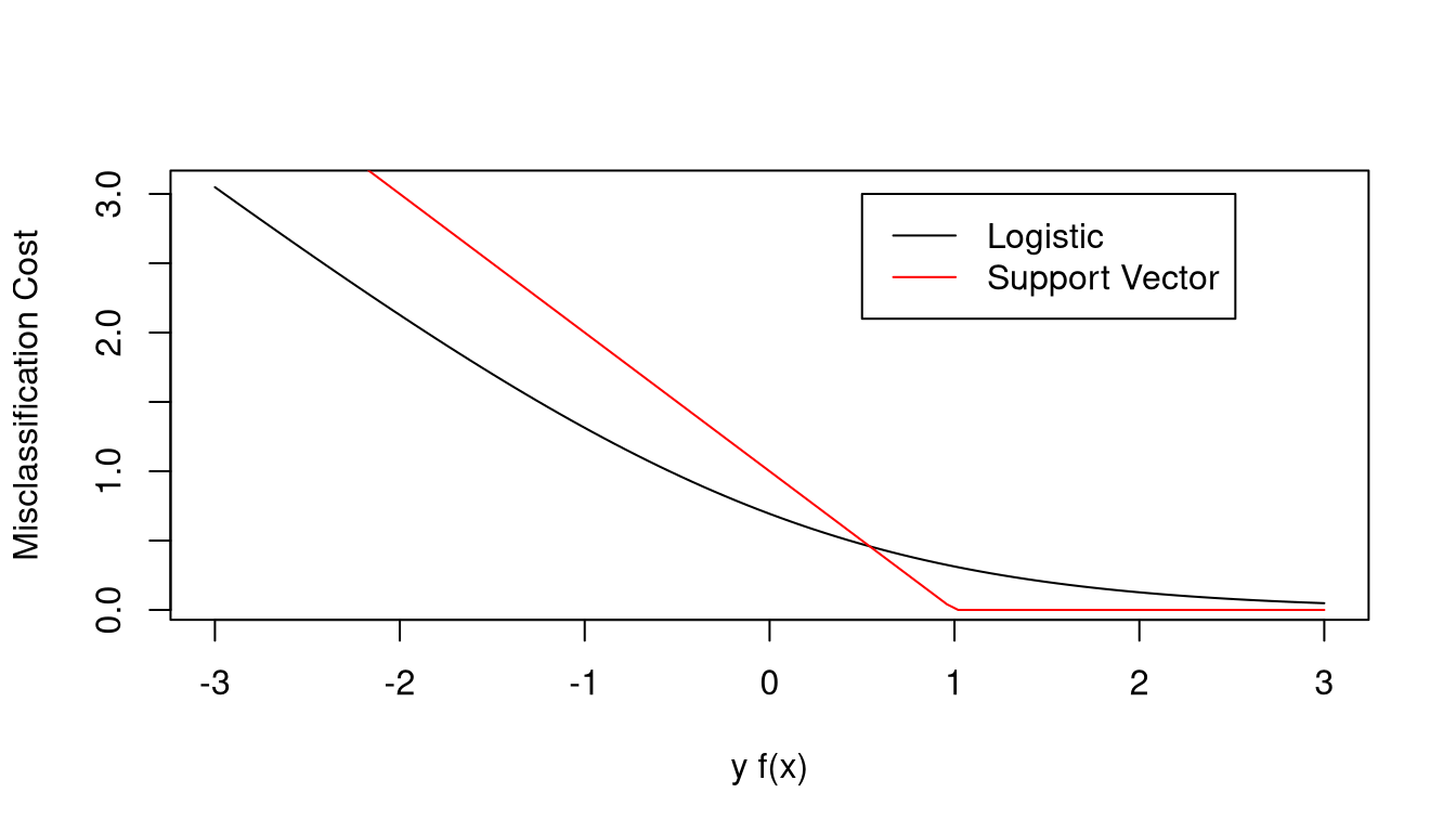
The support vector classifier loss function is sometimes called hinge loss.

Via rewriting in terms of equivalent convex optimization problems it can be shown that the minimizer \(\widehat{\beta}\) has the form

\[\begin{equation*} \widehat{\beta} = \sum_{i=1}^n \widehat{\alpha}_i y_i x_i \end{equation*}\]

for some values \(\widehat{\alpha}_i \in [0,1/(2\lambda)]\).

Therefore

\[\begin{equation*} \newcommand{\ip}[2]{\langle{#1},{#2}\rangle} \widehat{f}(x) = x^T\widehat{\beta} + \widehat{\beta_0} = \widehat{\beta_0} + \sum_{i=1}^n \widehat{\alpha}_i y_i x^T x_i = \widehat{\beta_0} + \sum_{i=1}^n \widehat{\alpha}_i y_i \langle{x},{x_i}\rangle \end{equation*}\]

The values of \(\widehat{\alpha_i}\) are only non-zero for \(x_i\) close to the plane \(f(x) = 0\).

These \(x_i\) are called support vectors.

8.5.2 The “Kernel Trick”

To allow for non-linear decision boundaries, we can use an extended feature set

\[ h(x_i) = (h_1(x_i),\dots,h_M(x_i)) \]

A linear boundary in \(\mathbb{R}^M\) maps down to a nonlinear boundary in \(\mathbb{R}^p\).

For example, for \(p=2\) and

\[ h(x) = (x_1, x_2, x_1 x_2, x_1^2, x_2^2) \]

then \(M=5\) and a linear boundary in \(\mathbb{R}^5\) maps down to a quadratic boundary in \(\mathbb{R}^2\).

The estimated classification function will be of the form

\[\begin{equation*} \widehat{f}(x) = \widehat{\beta}_0 + \sum_{i=1}^n \widehat{\alpha}_i y_i \langle{h(x)},{h(x_i)}\rangle = \widehat{\beta}_0 + \sum_{i=1}^n \widehat{\alpha}_i y_i K(x,x_i) \end{equation*}\]

where the kernel function \(K\) is

\[ K(x, x') = \langle{h(x)},{h(x')}\rangle \]

The kernel function is symmetric and positive semi-definite.

We do not need to specify \(h\) explicitly, only \(K\) is needed.

Any symmetric, positive semi-definite function can be used.

Some common choices:

\[\begin{align*} \renewcommand{\ip}[2]{\langle{#1},{#2}\rangle} \renewcommand{\Norm}[1]{\|{#1}\|} \text{$d$th degree polynimial:} & \qquad K(x,x') = (1+\langle{x},{x'}\rangle)^d\\ \text{radial basis:} & \qquad K(x,x') = \exp(-\|{x-x'}\|^2/c)\\ \text{neural network:}& \qquad K(x,x') = \text{tanh}(a\langle{x},{x'}\rangle+b) \end{align*}\]

The parameter \(\lambda\) in the optimization criterion is a regularization parameter. It can be chosen by cross-validation.

Particular kernels and their parameters also need to be chosen.

This is analogous/equivalent to choosing sets of basis functions.

Smoothing splines can be expressed in terms of kernels as well.

• This leads to reproducing kernel Hilbert spaces.

• This does not lead to the sparseness of the SVM approach.

8.5.3 An Artificial Example

Classify random data as above or below a parabola:

x1 <- runif(100)
x2 <- runif(100)
z <- ifelse(x2 > 2 * (x1 - .5)^2 + .5, 1, 0)
plot(x1, x2, col = ifelse(z, "red", "blue"))
x <- seq(0, 1, len = 101)
lines(x, 2 * (x - .5)^2 + .5, lty = 2)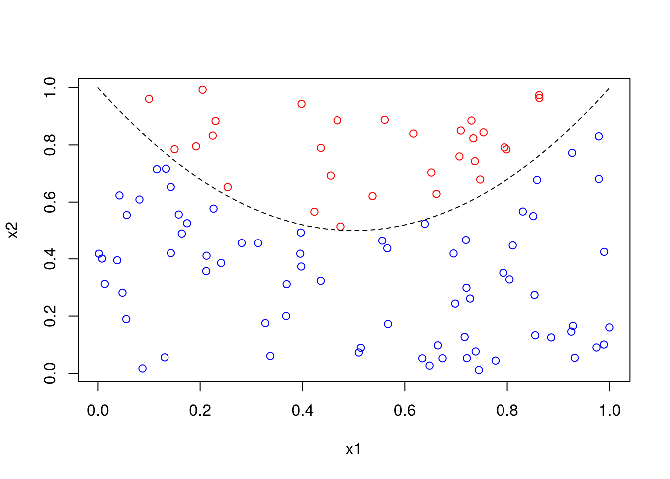

Fit a support vector classifier using \(\lambda = \frac{1}{2\text{cost}}\):

library(e1071)
fit <- svm(factor(z) ~ x1 + x2, cost = 10)
fit
## 
## Call:
## svm(formula = factor(z) ~ x1 + x2, cost = 10)
## 
## 
## Parameters:
##    SVM-Type:  C-classification 
##  SVM-Kernel:  radial 
##        cost:  10 
## 
## Number of Support Vectors:  15

plot(fit, data.frame(z=z,x1=x1,x2=x2),
          formula = x2 ~ x1, grid=100)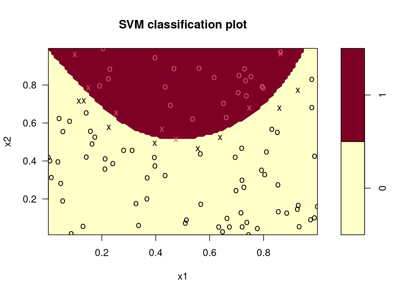

8.6 Neural Networks

Neural networks are flexible nonlinear models.

They are motivated by simple models for the working of neurons.

They connect input nodes to output nodes through one or more layers of hidden nodes

The simplest form is the feed-forward network with one hidden layer, inputs \(x_1,\dots,x_p\) and outputs \(y_1,\dots,y_k\).

A graphical representation:

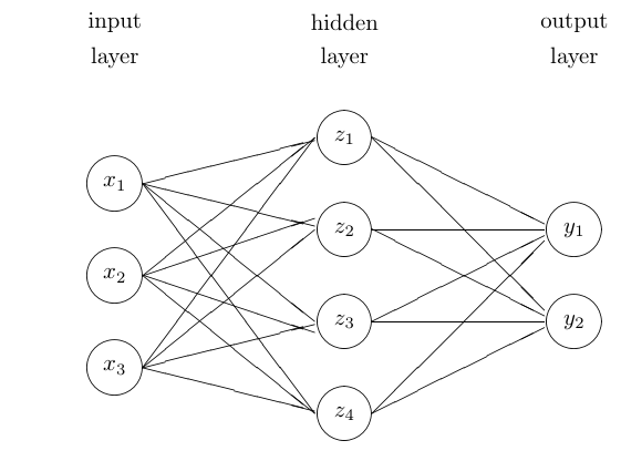
Mathematical form:

\[\begin{align*} z_m &= h(\alpha_{0m} + x^T \alpha_m)\\ t_k &= \beta_{0k} + z^T \beta_k\\ f_k(x) &= g_k(T) \end{align*}\]

The activation function \(h\) is often a sigmoidal function, like the logistic CDF

\[\begin{equation*} h(x) = 1 / (1 + e^{-x}) \end{equation*}\]

For regression there is usually one output with \(g_1(t)\) the identity function.

For binary classification there is usually one output with \(g_1(t) = 1 / (1 + e^{-t})\)

For \(k\)-class classification with \(k > 2\) usually there are \(k\) outputs, corresponding to binary class indicator data, with

\[\begin{equation*} g_k(t) = \frac{e^{t_k}}{\sum_j e^{t_j}} \end{equation*}\]

This is often called a softmax criterion.

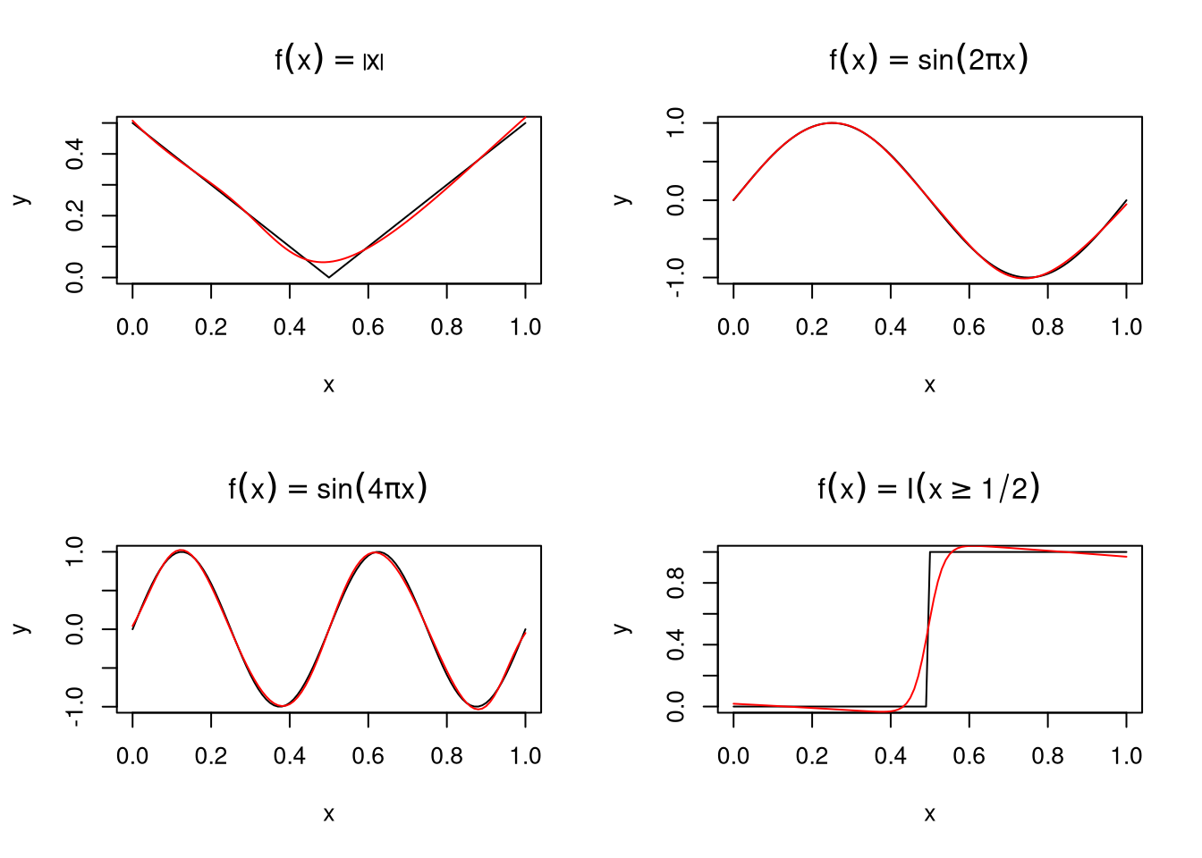
By increasing the size of the hidden layer \(M\) a neural network can uniformly approximate any continuous function on a compact set arbitrarily well.

Some examples, fit to \(n = 101\) data points using function neuralnet from package neuralnet with a hidden layer with \(M=5\) nodes:

Fitting is done by maximizing a log likelihood \(L(\alpha,\beta)\) assuming

• normal errors for regression

• a logistic model for classification

The likelihood is highly multimodal and the parameters are not identified

• relabeling hidden nodes does not change the model, for example

• random starting values are usually used

• parameters are not interpretable

If \(M\) is large enough to allow flexible fitting then over-fitting is a risk.

Regularization is used to control overfitting: a penalized log likelihood of the form

\[\begin{equation*} L(\alpha,\beta) - \lambda(\sum_m \|\alpha_m\|^2 + \sum_k \|\beta_k\|^2) \end{equation*}\]

is maximized.

• For this to make sense it is important to center and scale the features to have comparable units.

• This approach is referred to as weight decay and \(\lambda\) is the decay parameter.

As long as \(M\) is large enough and regularization is used, the specific value of \(M\) seems to matter little.

The weight decay parameter is often determined by \(N\)-fold cross validation, often with \(N=10\)

Because of the random starting points, results in repeated runs can differ.

• one option is to make several runs and pick the best fit

• another is to combine results from several runs by averaging or majority voting.

Fitting a neural net to the artificial data example:

library(neuralnet)
d <- data.frame(x1, x2, z)
fit <- neuralnet(z ~ x1 + x2, d, linear.output = FALSE, hidden = 10)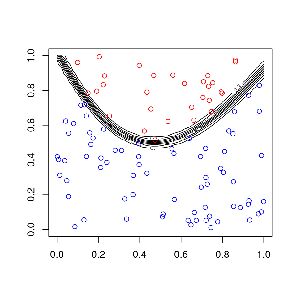

8.6.1 Example: Recognizing Handwritten Digits

Data consists of scanned ZIP code digist from the U.S. postal service.

Data is available at http://yann.lecun.com/exdb/mnist/ as a binary file.

Training data consist of a small number of original images, around 300, and additional images generated by random shifts.

Data are \(28 \times 28\) gray-scale images, along with labels.

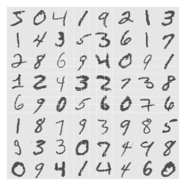
This has become a standard machine learning test example.

Data can be read into R using readBin.

The fit, using 6000 observations and \(M=100\) nodes in the hidden layer took 11.5 hours on r-lnx400:

library(nnet)
fit <- nnet(X, class.ind(lab), size = 100,
            MaxNWts = 100000, softmax = TRUE)

It produced a training misclassification rate of about 8% and a test misclassification rate of about 12%.

Other implementations are faster and better for large problems.

8.7 Deep Learning

Deep learning models are multi-level non-linear models

A supervised model with observed responses \(Y\) and features \(X\) with \(M\) layers would be \[\begin{equation*} Y \sim f_1(y|Z_1), Z_1 \sim f_2(z_1| Z_2), \dots, Z_M \sim f_M(z_M|X) \end{equation*}\] with \(Z_1, \dots, Z_M\) unobserved latent values.

An unsupervised model with observed features \(X\) would be

\[\begin{equation*} X \sim f_1(x|Z_1), Z_1 \sim f_2(z_1| Z_2), \dots, Z_M \sim f_M(z_M) \end{equation*}\]

These need to be nonlinear so they don’t collapse into one big linear model.

The layers are often viewed as capturing features at different levels of granularity.

For image classification these might be

• \(X\): pixel intensities

• \(Z_1\): edges

• \(Z_2\): object parts (e.g. eyes, noses)

• \(Z_3\): whole objects (e.g. faces)

Multi-layer, or deep, neural networks are one approach, that has become very successful.

Deep learning methods have become very successful in recent years due to a combination of increased computing power and algorithm improvements.

Some key algorithm developments include:

• Use of stochastic gradient descent for optimization.

• Backpropagation for efficient gradient evaluation.

• Using the piece-wise linear Rectified Linear Unit (ReLU) activation function \[\begin{equation*} \text{ReLU}(x) = \begin{cases} x & \text{if $x \ge 0$}\\ 0 & \text{otherwise.} \end{cases} \end{equation*}\]

• Specialized structures, such as convolutional and recurrent neural networks.

• Use of dropout, regularization, and early stopping to avoid over-fitting.

8.7.1 Stochastic Gradient Descent

Gradient descent for minimizing a function \(f\) tries to improve a current guess by taking a step in the direction of the negative gradient: \[\begin{equation*} x' = x - \eta \nabla f(x) \end{equation*}\]

The step size \(\eta\) is sometimes called the learning rate.

In one dimension the best step size near the minimum is \(1/f''(x)\).

A step size that is too small converges too slowly; a step size too large may not converge at all.

Line search is possible but may be expensive.

Using a fixed step size, with monitoring to avoid divergence, or using a slowly decreasing step size are common choices.

For a DNN the function to be minimized with respect to parameters \(A\) is typically of the form

\[\begin{equation*} \sum_{i=1}^n L_i(y_i, x_i, A) \end{equation*}\]

for large \(n\).

Computing function and gradient values for all \(n\) training cases can be very costly.

Stochastic gradient descent at each step chooses a random minibatch of \(B\) of the training cases and computes a new step based on the loss function for the minibatch.

The minibatch size can be as small as \(B = 1\).

Stochastic gradient descent optimizations are usually divided into epochs, with each epoch expected to use each training case once.

8.7.2 Backpropagation

Derivatives of the objective function are computed by the chain rule.

This is done most efficiently by working backwards; this corresponds to the reverse mode of automatic differentiation.

A DNN with two hidden layers can be represented as

\[\begin{equation*} F(x; A) = G(A_3 H_2(A_2 H_1(A_1 x))) \end{equation*}\]

If \(G\) is elementwise the identity, and the \(H_i\) are elementwise ReLU, then this is a piece-wise linear function of \(x\).

The computation of \(w = F(x; A)\) can be broken down into intermediate steps as \[\begin{align*} t_1 &= A_1 x & z_1 &= H_1(t_1)\\ t_2 &= A_2 z_1 & z_2 &= H_2(t_2)\\ t_3 &= A_3 z_2 & w &= G(t_3) \end{align*}\]

This is called forward propagation.

The gradient components are then computed in reverse, by backpropagation, as

\[\begin{align*} B_3 &= \nabla G(t_3) & \frac{\partial w}{\partial A_3} &= \nabla G(t_3) z_2 = B_3 z_2\\ B_2 &= B_3 A_3 \nabla H_2 (t_2) & \frac{\partial w}{\partial A_2} &= \nabla G(t_3) A_3 \nabla H_2 (t_2) z_1 = B_2 z_1\\ B_1 &= B_2 A_2 \nabla H_1 (t_1) & \frac{\partial w}{\partial A_1} &= \nabla G(t_3) A_3 \nabla H_2 (t_2) A_2 \nabla H_1(t_1) x = B_1 x \end{align*}\]

For ReLU activations the elements of \(\nabla H_i(t_i)\) will be 0 or 1.

For \(n\) parameters the computation will typically be of order \(O(n)\).

Many of the computations can be effectively parallelized.

8.7.3 Convolutional and Recurrent Neural Networks

In image processing features (pixel intensities) have a neighborhood structure.

A convolutional neural network uses one or more hidden layers that are:

• only locally connected;

• use the same parameters at each location.

A simple convolution layer might use a pixel and each of its 4 neighbors with

\[\begin{equation*} t = (a_1 R + a_2 L + a_3 U + a_4 D) z \end{equation*}\]

where, e.g.

\[\begin{equation*} R_{ij} = \begin{cases} 1 & \text{if pixel $i$ is immediately to the right of pixel $j$}\\ 0 & \text{otherwise}. \end{cases} \end{equation*}\]

With only a small nunber of parameters per layer it is feasible to add tens of layers.

Similarly, a recurrent neural network can be designed to handle temporal dependencies for time series or speech recognition.

8.7.4 Avoiding Over-Fitting

Both \(L_1\) and \(L_2\) regularization are used.

Another strategy is dropout:

• In each epoch keep a node with probability \(p\) and drop with probability \(1-p\).

• In the final fit multiply each node’s output by \(p\).

This simulates an ensemble method fitting many networks, but costs much less.

Random starts are an important component of fitting networks.

Stopping early, combined with random starts and randomness from stochastic gradient descent, is also thought to be an effective regularization.

Cross-validation during training can be used to determine when to stop.

8.7.5 Notes and References

Deep learning methods have been very successful in a number of areas, such as:

• Image classification and face recognition. AlexNet is a very successful image classifier.

• Google Translate is now based on a deep neural network approach.

• Speech recognition.

• Playing Go and chess.

Being able to effectively handle large data sets is an important consideration in this research.

Highly parallel GPU based and distributed architectures are often needed.

Some issues:

• Very large training data sets are often needed.

• In high dimensional problems having a high signal to noise ratio seems to be needed.

• Models can be very brittle – small data perturbations can lead to very wrong results.

• Biases in data will lead to biases in predictions. A probably harmless example deals with evaluating selfies in social media; there are much more serious examples.

Some R packages for deep learning include darch, deepnet, deepr, domino, h2o, keras.

Some references:

• A nice introduction was provided by Thomas Lumley in a 2019 Ihaka Lecture.

• deeplearning.net web site.

• Li Deng and Dong Yu (2014), Deep Learning: Methods and Applications.

• Charu Aggarwal (2018), Neural Networks and Deep Learning.

• A Primer on Deep Learning.

• A blog post on deep learning software in R.

• A nice simulator.

Some examples are available on line.

8.8 Mixture of Experts

Mixture models for prediction of \(y\) based on fearures \(x\) produce predictive distributions of the form \[\begin{equation*} f(y|x) = \sum_{i=1}^M f_i(y|x) \pi_i \end{equation*}\] with \(f_i\) depending on parameters that need to be learned from training data.

A generalization allows the mixing probabilities to depend on the features:

\[\begin{equation*} f(y|x) = \sum_{i=1}^M f_i(y|x) \pi_i(x) \end{equation*}\]

with \(f_i\) and \(\pi_i\) depending on parameters that need to be learned.

The \(f_i\) are referred to as experts, with different experts being better informed about different ranges of \(x\) values, and \(f\) this is called a mixture of experts.

Tree models can be viewed as a special case of a mixture of experts with \(\pi_i(x) \in \{0,1\}\).

The mixtures \(\pi_i\) can themselves be modeled as a mixture of experts. This is the hierarchical mixture of experts (HME) model.