Chapter 6 Density Estimation and Smoothing

6.1 Density Estimation

Suppose we have a random sample $X_1,\dots,X_n$ from a population with density $f$.

Nonparametric density estimation is useful if we want

to explore the data without a specific parametric model;
to assess the fit of a parametric model;
a compromise between a parametric and a fully non-parametric approach.

A simple method for estimating $f$ at a point $x$:

\[\begin{equation*} \widehat{f}_n(x) = \frac{\text{no. of $X_i$ in $[x-h,x+h]$}}{2hn} \end{equation*}\]

for some small value of $h$.

This estimator has bias

\[\begin{equation*} \text{Bias}(\widehat{f}_n(x)) = \frac{1}{2h}p_h(x) - f(x) \end{equation*}\]

and variance

\[ \text{Var}(\widehat{f}_n(x)) = \frac{p_h(x)(1-p_h(x))}{4h^2n} \]

with

\[\begin{equation*} p_h(x) = \int_{x-h}^{x+h}f(u)du \end{equation*}\]

If $f$ is continuous at $x$ and $f(x) > 0$, then as $h \to 0$

the bias tends to zero;
the variance tends to infinity.

Choosing a good value of $h$ involves a variance-bias tradeoff.

6.1.1 Kernel Density Estimation

The estimator $\widehat{f}_n(x)$ can be written as

\[\begin{equation*} \widehat{f}_n(x) = \frac{1}{nh}\sum_{i=1}^n K\left(\frac{x-x_i}{h}\right) \end{equation*}\]

with

\[\begin{equation*} K(u) = \begin{cases} 1/2 & \text{if $|u| < 1$}\\ 0 & \text{otherwise} \end{cases} \end{equation*}\]

Other kernel functions $K$ can be used; usually

$K$ is a density function
$K$ has mean zero
$K$ has positive, finite variance $\sigma_K^2$

Often $K$ is symmetric.

Common choices of $K$:

$K(u)$	Range	Name
$1/2$	\|$u$\| < 1	Uniform, Boxcar
$\frac{1}{\sqrt{2\pi}} e^{-u^2/2}$		Gaussian
1 - \|$u$\|	\|$u$\| < 1	Triangular
$\frac{3}{4}(1-u^2)$	\|$u$\| < 1	Epanechnikov
$\frac{15}{16}(1-u^2)^2$	\|$u$\| < 1	Biweight

6.1.2 Mean Square Error for Kernel Density Estimators

The bias and variance of a kernel density estimator are of the form

\[\begin{align*} \text{Bias}(\widehat{f}_n(x)) &= \frac{h^2\sigma_K^2 f''(x)}{2} + O(h^4)\\ \text{Var}(\widehat{f}_n(x)) &= \frac{f(x) R(K)}{nh} + o\left(\frac{1}{nh}\right) \end{align*}\]

with

\[\begin{equation*} R(g) = \int g(x)^2 dx \end{equation*}\]

if $h \to 0$ and $nh \to \infty$ and $f$ is reasonable.

The pointwise asymptotic mean square error is

\[\begin{equation*} \text{AMSE}(\widehat{f}_n(x)) = \frac{f(x) R(K)}{nh} + \frac{h^4\sigma_K^4 f''(x)^2}{4} \end{equation*}\]

and the asymptotic mean integrated square error is

\[\begin{equation*} \text{AMISE}(\widehat{f}_n) = \frac{R(K)}{nh} + \frac{h^4\sigma_K^4 R(f'')}{4} \end{equation*}\]

The resulting asymptotically optimal bandwidths $h$ are

\[\begin{align*} h_0(x) &= \left(\frac{f(x) R(K)}{\sigma_K^4 f''(x)^2}\right)^{1/5} n^{-1/5}\\ h_0 &= \left(\frac{R(K)}{\sigma_K^4 R(f'')}\right)^{1/5} n^{-1/5} \end{align*}\]

with optimal AMSE and AMISE

\[\begin{align*} \text{AMSE}_0(\widehat{f}_n(x)) &= \frac{5}{4}(\sigma_K f(x) R(K))^{4/5} f''(x)^{2/5} n^{-4/5}\\ \text{AMISE}_0(\widehat{f}_n) &= \frac{5}{4}(\sigma_K R(K))^{4/5} R(f'')^{1/5} n^{-4/5} \end{align*}\]

6.1.3 Choosing a Bandwidth

One way to chose a bandwidth is to target a particular family, such as a Gaussian $f$:

The optimal bandwidth for minimizing AMISE when $f$ is Gaussian and $K$ is Gaussian

\[h_0 = 1.059 \sigma n^{-1/5}\]
$\sigma$ can be estimated using $S$ or the interquartile range

The default for density in R is

\[0.9 \times \min(S, \text{IQR}/1.34)n^{-1/5}\]

based on a suggestion of Silverman (1986, pp 45–47).

This can often serve as a reasonable starting point.

It does not adapt to information in the data that suggests departures from normality.

So-called plug-in methods estimate $R(f'')$ to obtain

\[\begin{equation*} \widehat{h} = \left(\frac{R(K)}{\sigma_K^4 \widehat{R(f'')}}\right)^{1/5} n^{-1/5} \end{equation*}\]

The Sheather-Jones method uses a different bandwidth (and kernel?) to estimate $\widehat{f}$ and then estimates $R(f'')$ by $R(\widehat{f}'')$.

Specifying bw="SJ" in R’s density uses the Sheather-Jones method.

There are two variants:

SJ-dpi: direct plug-in
SJ-ste: solve the equation

The default for bw="SJ" is ste.

Other approaches based on leave-one-out cross-validation are available.

Many of these are available as options in R’s density and/or other density estimation functions available in R packages.

Variable bandwidth approaches can be based on pilot estimates of the density produced with simpler fixed bandwidth rules.

6.1.4 Example: Durations of Eruptions of Old Faithful

Based on an example in Venables and Ripley (2002).

Durations, in minutes, of 299 consecutive eruptions of Old Faithful were recorded.

The data are available as data set geyser in package MASS.

Some density estimates are produced by

library(MASS)
data(geyser)
truehist(geyser$duration,nbin=25,col="lightgrey")
lines(density(geyser$duration))
lines(density(geyser$duration,bw="SJ"), col="red")
lines(density(geyser$duration,bw="SJ-dpi"), col="blue")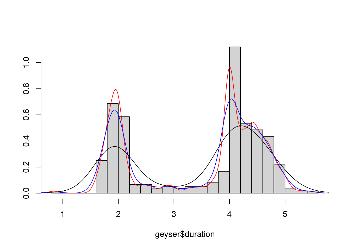

Animation can be a useful way of understanding the effect of smoothing parameter choice.

See files tkdens.R, shinydens.R, and geyser.R in the class examples directory.

More examples are in the same directory in smoothex.Rmd.

6.1.5 Issues and Notes

Kernel methods do not work well at boundaries of bounded regions.

Transforming to unbounded regions is often a good alternative.

Variability can be assessed by asymptotic methods or by bootstrapping.

A crude MCMC bootstrap animation:

data(geyser, package = "MASS")
g <- geyser$duration
for (i in 1:1000) {
    g[sample(299,1)] <- geyser$duration[sample(299,1)]
    plot(density(g,bw="SJ"),ylim=c(0,1.2),xlim=c(0,6))
    Sys.sleep(1/30)
}

Computation is often done with equally spaced bins and fast Fourier transforms.

Methods that adjust bandwidth locally can be used.

Some of these methods are based on nearest-neighbor fits and local polynomial fits.

Spline based methods can be used on the log scale; the logspline package implements one approach.

6.1.6 Density Estimation in Higher Dimensions

Kernel density estimation can in principle be used in any number of dimensions.

Usually a $d$-dimensional kernel $K_d$ of the product form

\[\begin{equation*} K_d(u) = \prod_{i=1}^d K_1(u_i) \end{equation*}\]

is used.

The kernel density estimate is then

\[\begin{equation*} \widehat{f}_n(x) = \frac{1}{n\det(H)}\sum_{i=1}^n K(H^{-1}(x-x_i)) \end{equation*}\]

for some matrix $H$.

Suppose $H = hA$ where $\det(A)=1$.

The asymptotic mean integrated square error is of the form

\[\begin{equation*} \text{AMISE} = \frac{R(K)}{nh^d} + \frac{h^4}{4}\int (\text{trace}(AA^T \nabla^2f(x)))^2dx \end{equation*}\]

and therefore the optimal bandwidth and AMISE are of the form

\[\begin{align*} h_0 &= O(n^{-1/(d+4)})\\ \text{AMISE}_0 &= O(n^{-4/(d+4)}) \end{align*}\]

Convergence is very slow if $d$ is more than 2 or 3 since most of higher dimensional space will be empty.

This is known as the curse of dimensionality.

Density estimates in two dimensions can be visualized using perspective plots, surface plots, image plots, and contour plots.

Higher dimensional estimates can often only be visualized by conditioning, or slicing.

The kde2d function in package MASS provides two-dimensional kernel density estimates; an alternative is bkde2D in package KernSmooth.

The kde3d function in the misc3d package provides three-dimensional kernel density estimates.

6.1.7 Example: Eruptions of Old Faithful

In addition to duration times, waiting times, in minutes, until the following eruption were recorded.

The duration of an eruption can be used to predict the waiting time until the next eruption.

A modified data frame containing the previous duration is constructed by

geyser2<-data.frame(as.data.frame(geyser[-1,]),
                    pduration=geyser$duration[-299])

Estimates of the joint density of previous eruption duration and waiting time are computed by

kd1 <- with(geyser2,
            kde2d(pduration, waiting,
                  n = 50,
                  lims = c(0.5, 6, 40, 110)))
with(geyser2, plot(pduration, waiting,
                   col = "blue",
                   xlab = "Previous Duration",
                   ylab = "Waiting"))
contour(kd1, col = "grey10", add = TRUE)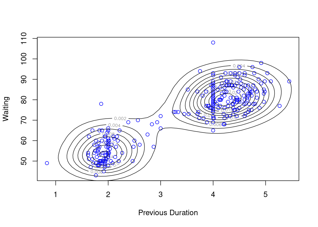

kd2 <- with(geyser2,
            kde2d(pduration, waiting,
                  n = 50,
                  lims = c(0.5, 6, 40, 110),
                  h = c(width.SJ(pduration),
                        width.SJ(waiting))))
with(geyser2, plot(pduration, waiting,
                   col = "blue",
                   xlab = "Previous Duration",
                   ylab = "Waiting"))
contour(kd2, col = "grey10", add = TRUE)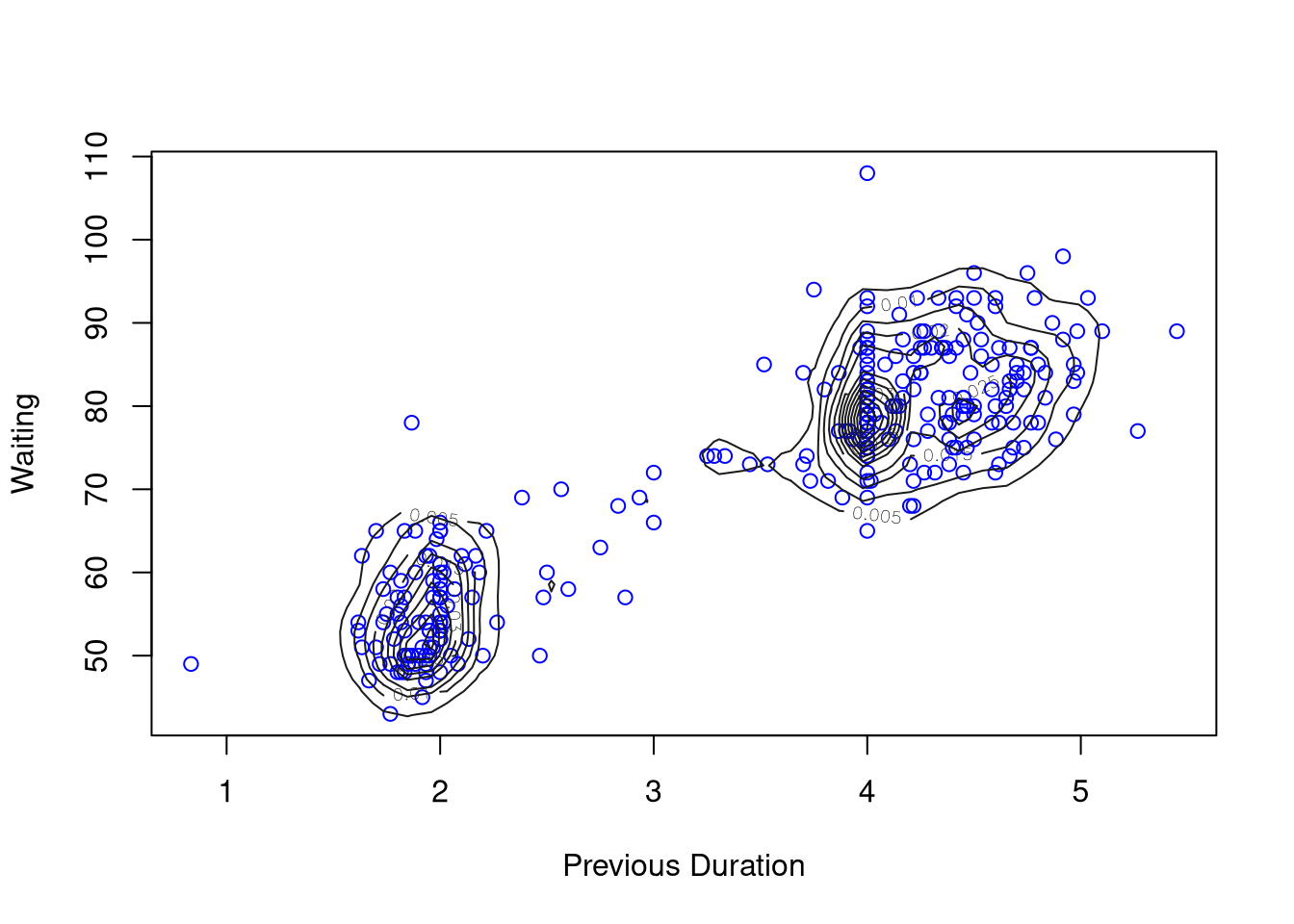

Rounding of some durations to 2 and 4 minutes can be seen.

6.1.8 Visualizing Density Estimates

Some examples are given in geyser.R and kd3.R in in the class examples directory.

Animation can be a useful way of understanding the effect of smoothing parameter choice.

Bootstrap animation can help in visualizing uncertainty.

For 2D estimates, options include

perspective plots
contour plots
image plots, with or without contours

For 3D estimates contour plots are the main option

Example: Data and contours for mixture of three trivariate normals and two bandwidths

Figure 6.1: BW = 0.2

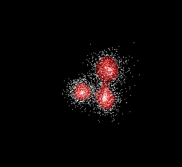
Figure 6.2: BW = 0.5

An example of using 3D density estimates with the quakes data is available.

6.2 Smoothing

6.2.1 Kernel Smoothing and Local Regression

A simple non-parametric regression model is

\[\begin{equation*} Y_i = m(x_i) + \epsilon_i \end{equation*}\]

with $m$ a smooth mean function.

A kernel density estimator of the conditional density $f(y|x)$ is

\[\begin{equation*} \widehat{f}_n(y|x) = \frac{\frac{1}{nh^2} \sum K\left(\frac{x-x_i}{h}\right)K\left(\frac{y-y_i}{h}\right)} {\frac{1}{nh}\sum K\left(\frac{x-x_i}{h}\right)} = \frac{1}{h} \frac{\sum K\left(\frac{x-x_i}{h}\right)K\left(\frac{y-y_i}{h}\right)} {\sum K\left(\frac{x-x_i}{h}\right)} \end{equation*}\]

Assuming $K$ has mean zero, an estimate of the conditional mean is

\[\begin{align*} \widehat{m}_n(x) &= \int y \widehat{f}_n(y|x) dy = \frac{\sum K\left(\frac{x-x_i}{h}\right) \int y \frac{1}{h}K\left(\frac{y-y_i}{h}\right)dy} {\sum K\left(\frac{x-x_i}{h}\right)}\\ &= \frac{\sum K\left(\frac{x-x_i}{h}\right) y_i} {\sum K\left(\frac{x-x_i}{h}\right)} = \sum w_i(x) y_i \end{align*}\]

This is the Nadaraya-Watson estimator.

This estimator can also be viewed as the result of a locally constant fit: $\widehat{m}_n(x)$ is the value $\beta_0$ that minimizes

\[\begin{equation*} \sum w_i(x) (y_i - \beta_0)^2 \end{equation*}\]

Higher degree local polynomial estimators estimate $m(x)$ by minimizing

\[\begin{equation*} \sum w_i(x) (y_i - \beta_0 - \beta_1 (x-x_i) - \dots - \beta_p (x-x_i)^p)^2 \end{equation*}\]

Odd values of $p$ have advantages, and $p=1$, local linear fitting, generally works well.

Local cubic fits, $p=3$, are also used.

Problems exist near the boundary; these tend to be worse for higher degree fits.

Bandwidth can be chosen globally or locally.

A common local choice uses a fraction of nearest neighbors in the $x$ direction.

Automatic choices can use estimates of $\sigma$ and function roughness and plug in to asymptotic approximate mean square errors.

Cross-validation can also be used; it often undersmooths.

Autocorrelation creates an identifiability problem.

Software available in R includes

ksmooth for compatibility with S (but much faster).
locpoly for fitting and dpill for bandwidth selection in package KernSmooth.
lowess and loess for nearest neighbor based methods; also try to robustify.
supsmu, Friedman’s super smoother, a very fast smoother.
package locfit on CRAN

Some are also available as stand-alone code.

6.2.2 Spline Smoothing

Given data $(x_1, y_1),\dots,(x_n,y_n)$ with $x_i \in [a,b]$ one way to fit a smooth mean function is to choose $m$ to minimize

\[\begin{equation*} S(m,\lambda) = \sum (y_i - m(x_i))^2 + \lambda \int_a^b m''(u)^2 du \end{equation*}\]

The term $\lambda \int_a^b m''(u)^2 du$ is a roughness penalty.

Among all twice continuously differentiable functions on $[a,b]$ this is minimized by a natural cubic spline with knots at the $x_i$.

This minimizer is called a smoothing spline.

A cubic spline is a function $g$ on an interval $[a,b]$ such that for some knots $t_i$ with $a = t_0 < t_1 < \dots < t_{n+1} = b$

on $(t_{i-1}, t_i)$ the function $g$ is a cubic polynomial
at $t_1,\dots,t_n$ the function values, first and second derivatives are continuous.

A cubic spline is natural if the second and third derivatives are zero at $a$ and $b$.

A natural cubic spline is linear on $[a,t_1]$ and $[t_n,b]$.

For a given $\lambda$ the smoothing spline is a linear estimator.

The set of equations to be solved is large but banded.

The fitted values $\widehat{m}_n(x_i,\lambda)$ can be viewed as

\[\begin{equation*} \widehat{m}_n(x,\lambda) = A(\lambda) y \end{equation*}\]

where $A(\lambda)$ is the smoothing matrix or hat matrix for the linear fit.

The function smooth.spline implements smoothing splines in R.

6.2.3 Example: Old Faithful Eruptions

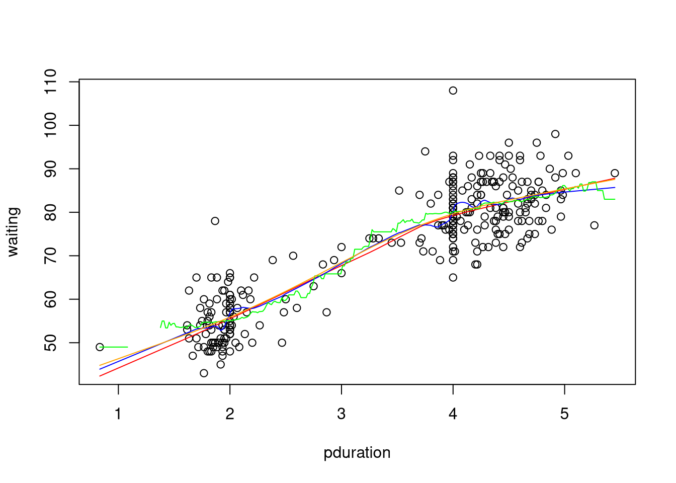
A nonparametric fit of waiting time to previous duration may be useful in predicting the time of the next eruption.

The different smoothing methods considered produce the following:

with(geyser2, {
     plot(pduration,waiting)
     lines(lowess(pduration,waiting), col="red")
     lines(supsmu(pduration,waiting), col="blue")
     lines(ksmooth(pduration,waiting), col="green")
     lines(smooth.spline(pduration,waiting), col="orange")
})

An animated version of the smoothing spline available on line shows the effect of varying the smoothing parameter.

6.2.4 Degrees of Freedom of a Linear Smoother

For a linear regression fit with hat matrix

\[\begin{equation*} H = X (X^TX)^{-1}X^T \end{equation*}\]

and full rank regressor matrix $X$

\[\begin{equation*} \text{tr}(H) = \text{number of fitted parameters} = \text{degrees of freedom of fit} \end{equation*}\]

By analogy define the degrees of freedom of a linear smoother as

\[\begin{equation*} \text{df}_\text{fit} = \text{tr}(A(\lambda)) \end{equation*}\]

For the geyser data, the degrees of freedom of a smoothing spline fit with the default bandwidth selection rule are

with(geyser2, sum(smooth.spline(pduration, waiting)$lev))
## [1] 4.169841
with(geyser2, smooth.spline(pduration, waiting))$df
## [1] 4.169841

For residual degrees of freedom the definition usually used is

\[\begin{equation*} \text{df}_\text{res} = n - 2 \text{tr}(A(\lambda)) + \text{tr}(A(\lambda)A(\lambda)^T) \end{equation*}\]

Assuming constant error variance, a possible estimate is

\[\begin{equation*} \widehat{\sigma}_\epsilon^2 = \frac{\sum (y_i-\widehat{m}_n(x_i,\lambda))^2}{\text{df}_\text{res}(\lambda)} = \frac{\text{RSS}(\lambda)}{\text{df}_\text{res}(\lambda)} \end{equation*}\]

The simpler estimator

\[\begin{equation*} \widehat{\sigma}_\epsilon^2 = \frac{\text{RSS}(\lambda)}{\text{tr}(I-A(\lambda))} = \frac{\text{RSS}(\lambda)}{n - \text{df}_\text{fit}} \end{equation*}\]

is also used.

To reduce bias it may make sense to use a rougher smooth for variance estimation than for mean function estimation.

6.2.5 Choosing Smoothing Parameters for Linear Smoothers

Many smoothing methods are linear for a given value of a smoothing parameter $\lambda$.

Choice of the smoothing parameter $\lambda$ can be based on leave-one-out cross-validation, i.e. minimizing the cross-validation score

\[\begin{equation*} \text{CV}(\lambda) = \frac{1}{n} \sum (y_i - \widehat{m}_n^{(-i)}(x_i, \lambda))^2 \end{equation*}\]

If the smoother satisfies (at least approximately)

\[\begin{equation*} \widehat{m}_n^{(-i)}(x_i, \lambda) = \frac{\sum_{j \neq i} A(\lambda)_{ij} y_j}{\sum_{j \neq i} A(\lambda)_{ij}} \end{equation*}\]

and for all $i$

\[\begin{equation*} \sum_{j=1}^n A(\lambda)_{ij} = 1 \end{equation*}\]

then the cross-validation score can be computed as

\[\begin{equation*} \text{CV}(\lambda) = \frac{1}{n}\sum \left(\frac{y_i - \widehat{m}_n(x_i, \lambda)}{1-A_{ii}(\lambda)}\right)^2 \end{equation*}\]

The generalized cross-validation criterion, or GCV, uses average leverage values:

\[\begin{equation*} \text{GCV}(\lambda) = \frac{1}{n}\sum \left(\frac{y_i - \widehat{m}_n(x_i, \lambda)} {1-n^{-1}\text{trace}(A(\lambda))}\right)^2 \end{equation*}\]

The original motivation for GCV was computational; with better algorithms this is no longer an issue.

An alternative motivation for GCV:

For an orthogonal transformation $Q$ one can consider fitting $y_Q=QY$ with $A_Q(\lambda) = Q A(\lambda) Q^T$.
Coefficient estimates and $SS_\text{res}$ are the same for all $Q$, but the CV score is not.
One can choose an orthogonal transformation such that the diagonal elements of $A_Q(\lambda)$ are constant.
For any such $Q$ we have \[A_Q(\lambda)_{ii} = n^{-1} \text{trace}(A_Q(\lambda)) = n^{-1} \text{trace}(A(\lambda))\]

Despite the name, GCV does not generalize CV.

Both CV and GCV have a tendency to undersmooth.

For the geyser data this code extracts and plots GCV and CV values:

with(geyser2, {
    lambda <- seq(0.5,2,len=30)
    f <- function(s, cv = FALSE)
        smooth.spline(pduration, waiting,
                      spar = s, cv = cv)$cv
    gcv <- sapply(lambda, f) 
    cv <- sapply(lambda, f, TRUE) 
    plot(lambda, gcv, type="l")
    lines(lambda, cv, col="blue")
})

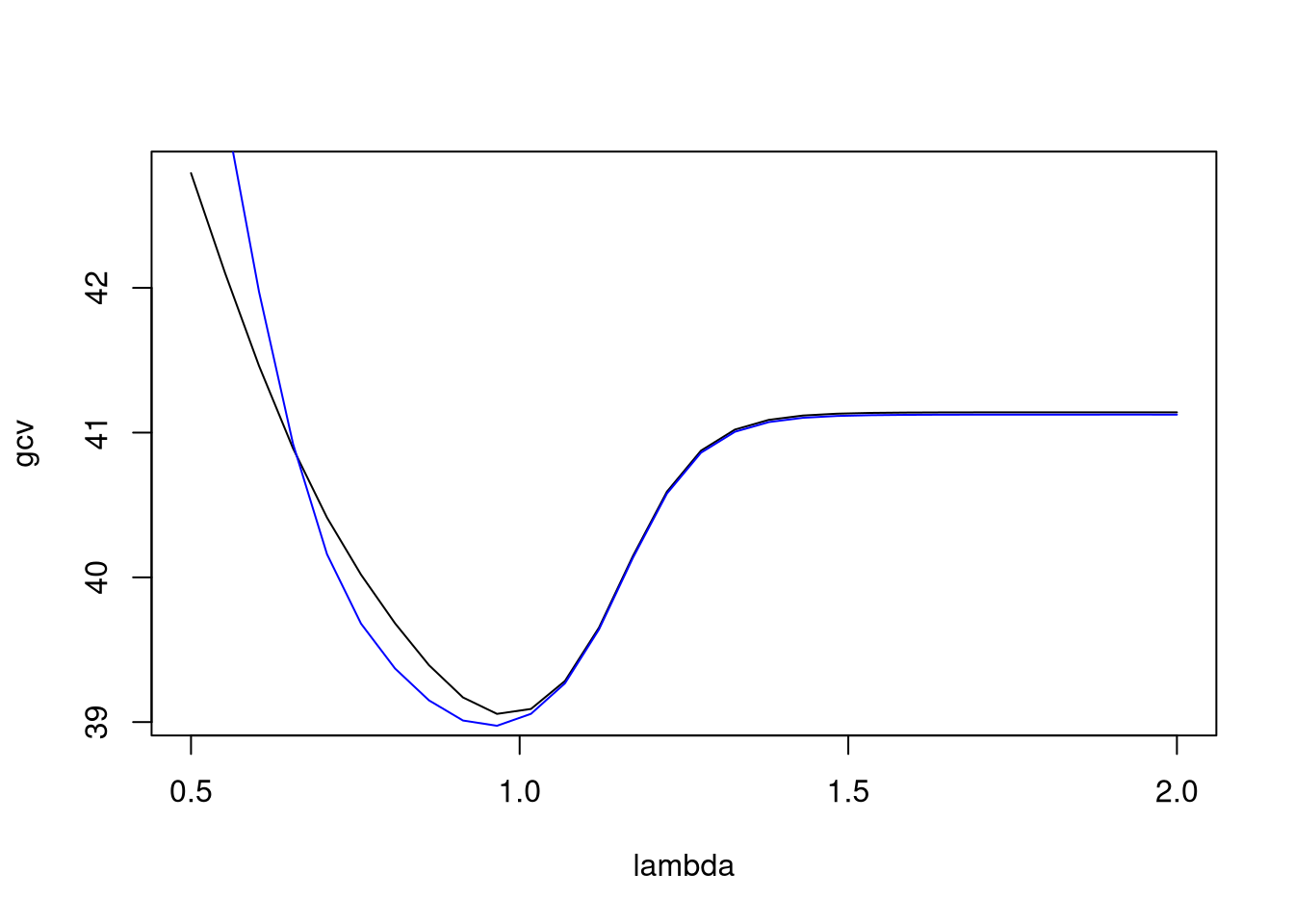
Both criteria select a value of $\lambda$ close to 1.

Other smoothing parameter selection criteria include

Mallows $C_p$, \[C_p = \text{RSS}(\lambda) + 2 \widehat{\sigma}_\epsilon^2\text{df}_\text{fit}(\lambda)\]
Akaike’s information criterion (AIC) \[\text{AIC}(\lambda) = \log\{\text{RSS}(\lambda)\} + 2\text{df}_\text{fit}(\lambda)/n\]
Corrected AIC of Hurvich, Simonoff, and Tsai (1998) \[\text{AIC}_C(\lambda) = \log\{\text{RSS}(\lambda)\} + \frac{2(\text{df}_\text{fit}(\lambda)+1)}{n-\text{df}_\text{fit}(\lambda)-2}\]

6.2.6 Spline Representations

Splines can be written in terms of many different bases:

B-splines;
truncated power basis;
radial or thin plate basis.

Some are more useful numerically, others have interpretational advantages.

One useful basis for a cubic spline with knots $\{\kappa_1,\dots,\kappa_K\}$ is the radial basis or thin plate basis

\[\begin{equation*} 1, x, |x-\kappa_1|^3, \dots, |x-\kappa_K|^3 \end{equation*}\]

More generally, a basis for splines of order $2m-1$ is

\[\begin{equation*} 1, x, \dots,x^{m-1},|x-\kappa_1|^{2m-1}, \dots, |x-\kappa_K|^{2m-1} \end{equation*}\]

for $m = 1, 2, 3, \dots$.

$m = 2$ produces cubic splines
$m = 1$ produces linear splines

In terms of this basis a spline is a function of the form

\[\begin{equation*} f(x) = \sum_{j=0}^{m-1} \beta_j x^j + \sum_{k=1}^K \delta_k |x-\kappa_k|^{2m-1} \end{equation*}\]

References:

P. J. Green and B. W. Silverman (1994). Nonparametric Regression and Generalied Linear Models

D. Ruppert, M. P. Wand, and R. J. Carroll (2003). Semiparametric Regression. SemiPar is an R package implementing the methods of this book.

G. Wahba (1990). Spline Models for Observational Data.

S. Wood (2017). Generalized Additive Models: An Introduction with R, 2nd Ed.. This is related to the mgcv package.

A generic form for the fitted values is

\[\begin{equation*} \widehat{y} = X_0 \beta + X_1 \delta. \end{equation*}\]

Regression splines refers to models with a small number of knots $K$ fit by ordinary least squares, i.e. by choosing $\beta, \delta$ to minimize

\[\|{y - X_0\beta - X_1\delta}\|^2\]

Penalized spline smoothing fits models with a larger number of knots subject to a quadratic constraint

\[\delta^T D \delta \le C\]

for a positive definite $D$ and some $C$.

Equivalently, by a Lagrange multiplier argument, the solution minimizes the penalized least squares criterion

\[\|{y - X_0\beta - X_1\delta}\|^2 + \lambda \delta^T D \delta\]

for some $\lambda > 0$.

A common form of $D$, that is not positive definite, is

\[D = \underset{1 \le i,j \le K}{\left[|\kappa_i-\kappa_j|^{2m-1}\right]}\]

A variant uses

\[D = \Omega^{1/2} (\Omega^{1/2})^T\]

with

\[\Omega = \underset{1 \le i,j \le K}{\left[|\kappa_i-\kappa_j|^{2m-1}\right]}\]

where the principal square root $M^{1/2}$ of a matrix $M$ with SVD

\[M = U \text{diag}(d) V^T\]

is defined as

\[M^{1/2} = U \text{diag}(\sqrt{d}) V^T\]

This form ensures that $D$ is at least positive semi-definite.

Smoothing splines are penalized splines of degree $2m-1=3$ with knots $\kappa_i = x_i$ and

\[D = \underset{1 \le i,j \le n}{\left[|\kappa_i-\kappa_j|^3\right]}\]

and the added natural boundary constraint

\[ X_0^T \delta = 0 \]

For a natural cubic spline

\[ \int g''(t)^2 dt = \delta^T D \delta \]

The quadratic form $\delta^T D \delta$ is strictly positive definite on the subspace defined by $X_0^T\delta = 0$.

Penalized splines can often approximate smoothing splines well using far fewer knots.

The detailed placement of knots and their number is usually not critical as long as there are enough.

Simple default rules that often work well (Ruppert, Wand, and Carroll 2003):

knot locations: \[ \kappa_k = \left(\frac{k+1}{K+2}\right)\text{th sample quantile of unique $x_i$}\]
number of knots: \[K = \min\left(\text{$\frac{1}{4} \times$ number of unique $x_i$, 35}\right)\]

The SemiPar package actually seems to use the default \[K = \max\left(\text{$\frac{1}{4} \times$ number of unique $x_i$, 20}\right)\]

More sophisticated methods for choosing number and location of knots are possible but not emphasized in the penalized spline literature at this point.

6.2.7 A Useful Computational Device

To minimize

\[ \|{Y - X_0\beta - X_1\delta}\|^2 + \lambda \delta^T D \delta \]

for a given $\lambda$, suppose $B$ satisties

\[ \lambda D = B^T B \]

and

\[\begin{align*} Y^* &= \begin{bmatrix} Y\\ 0 \end{bmatrix} & X^* &= \begin{bmatrix} X_0 & X_1\\ 0 & B \end{bmatrix} & \beta^* = \begin{bmatrix} \beta\\ \delta \end{bmatrix} \end{align*}\]

Then

\[\|{Y^* - X^*\beta^*}\|^2 = \|{Y - X_0\beta - X_1\delta}\|^2 + \lambda \delta^T D \delta\]

So $\widehat{\beta}$ and $\widehat{\delta}$ can be computed by finding the OLS coefficients for the regression of $Y^*$ on $X^*$.

6.2.8 Penalized Splines and Mixed Models

For strictly positive definite $D$ and a given $\lambda$, minimizing the objective function

\[ \|{y - X_0\beta - X_1\delta}\|^2 + \lambda \delta^T D \delta \]

is equivalent to maximizing the log likelihood for the mixed model

\[ Y = X_0\beta + X_1\delta + \epsilon \]

with fixed effects parameters $\beta$ and

\[\begin{align*} \epsilon &\sim \text{N}(0, \sigma_\epsilon^2 I)\\ \delta &\sim \text{N}(0, \sigma_\delta^2 D^{-1})\\ \lambda &= \sigma_\epsilon^2 / \sigma_\delta^2 \end{align*}\]

with $\lambda$ known.

Some consequences:

The penalized spline fit at $x$ is the BLUP for the mixed model with known mixed effects covariance structure.
Linear mixed model software can be used to fit penalized spline models (the R package SemiPar does this).
The smoothing parameter $\lambda$ can be estimated using ML or REML estimates of $\sigma_\epsilon^2$ and $\sigma_\delta^2$ from the linear mixed model.
Interval estimation/testing formulations from mixed models can be used.

Additional consequences:

The criterion has a Bayesian interpretation.
Extension to models containing smoothing and mixed effects are immediate.
Extension to generalized linear models can use GLMM methodology.

6.2.9 Example: Old Faithful Eruptions

Using the function spm from SemiPar a penalized spline model can be fit with

library(SemiPar)
attach(geyser2) # needed because of flaws in spm implementation
summary(spm(waiting ~ f(pduration)))
## 
## 
## Summary for non-linear components:
## 
##                 df spar knots
## f(pduration) 4.573  2.9    28
## 
## Note this includes 1 df for the intercept.

The plot method for the spm result produces a plot with pointwise error bars:

plot(spm(waiting ~ f(pduration)), ylim = range(waiting))
points(pduration, waiting)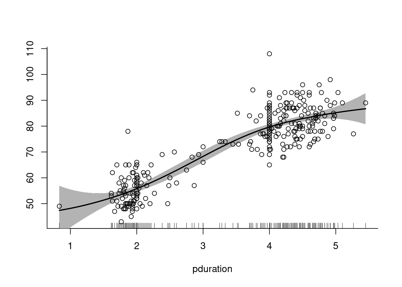

A fit using mgcv:

library(mgcv)
gam.fit <- gam(waiting ~ s(pduration), data = geyser2)
summary(gam.fit)
## 
## Family: gaussian 
## Link function: identity 
## 
## Formula:
## waiting ~ s(pduration)
## 
## Parametric coefficients:
##             Estimate Std. Error t value Pr(>|t|)    
## (Intercept)  72.2886     0.3594   201.1   <2e-16 ***
## ---
## Signif. codes:  
## 0 '***' 0.001 '**' 0.01 '*' 0.05 '.' 0.1 ' ' 1
## 
## Approximate significance of smooth terms:
##                edf Ref.df     F p-value    
## s(pduration) 3.149  3.987 299.8  <2e-16 ***
## ---
## Signif. codes:  
## 0 '***' 0.001 '**' 0.01 '*' 0.05 '.' 0.1 ' ' 1
## 
## R-sq.(adj) =  0.801   Deviance explained = 80.3%
## GCV = 39.046  Scale est. = 38.503    n = 298

A plot of the smooth component with the mean-adjusted waiting times is produced by

plot(gam.fit)
with(geyser2, points(pduration, waiting - mean(waiting)))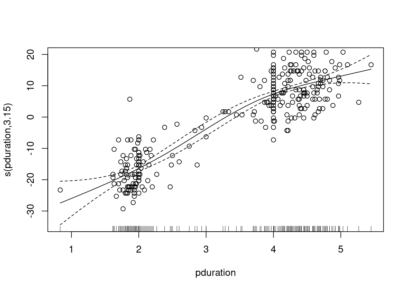

6.2.10 Smoothing with Multiple Predictors

Many methods have natural generalizations

All suffer from the curse of dimensionality.

Generalizations to two or three variables can work reasonably.

Local polynomial fits can be generalized to $p$ predictors.

loess is designed to handle multiple predictors, in principle at least.

Spline methods can be generalized in two ways:

tensor product splines use all possible products of single variable spline bases.
thin plate splines generalize the radial basis representation.

A thin plate spline of order $m$ in $d$ dimensions is of the form

\[\begin{equation*} f(x) = \sum_{i=1}^M \beta_i \phi_i(x) + \sum_{k=1}^K\delta_k r(x-\kappa_k) \end{equation*}\]

with

\[ r(u) = \begin{cases} \|{u}\|^{2m-d} & \text{for $d$ odd}\\ \|{u}\|^{2m-d}\log\|{u}\| & \text{for $d$ even}\\ \end{cases} \]

and where the $\phi_i$ are a basis for the space of polynomials of total degree $\le m - 1$ in $d$ variables.

The dimension of this space is

\[ M = \binom{d+m-1}{d} \]

If $d = 2, m = 2$ then $M = 3$ and a basis is

\[ \phi_1(x) = 1, \phi_2(x) = x_1, \phi_3(x) = x_2 \]

6.2.11 Penalized Thin Plate Splines

Penalized thin plate splines usually use a penalty with

\[\begin{equation*} D = \Omega^{1/2} (\Omega^{1/2})^T \end{equation*}\]

where

\[\begin{equation*} \Omega = \underset{1 \le i,j \le K}{\left[r(\kappa_i-\kappa_j)\right]} \end{equation*}\]

This corresponds at least approximately to using a squared derivative penalty.

Simple knot selection rules are harder for $d > 1$.

Some approaches:

space-filling designs (Nychka and Saltzman, 1998);
clustering algorithms, such as clara.

6.2.12 Multivariate Smoothing Splines

The bivariate smoothing spline objective of minimizing

\[\begin{equation*} \sum (y_i - g(x_i))^2 + \lambda J(g) \end{equation*}\]

with

\[\begin{equation*} J(g) = \int \int \left(\frac{\partial^2 g}{\partial x_1^2}\right)^2 + 2 \left(\frac{\partial^2 g}{\partial x_1\partial x_2}\right)^2 + \left(\frac{\partial^2 g}{\partial x_2^2}\right)^2 dx_1 dx_2 \end{equation*}\]

is minimized by a thin plate spline with knots at the $x_i$ and a constraint on the $\delta_k$ analogous to the natural spline constraint.

Scaling of variables needs to be addressed.

Thin-plate spline smoothing is closely related to kriging.

The general smoothing spline uses

\[\begin{equation*} D = X_1 = [r(\kappa_i - \kappa_i)] \end{equation*}\]

with the constraint $X_0^T\delta = 0$.

Challenge: The linear system to be solved for each $\lambda$ value to fit a smoothing spline is large and not sparse.

6.2.13 Thin Plate Regression Splines

Wood (2017) advocates an approach called thin plate regression splines that is implemented in the mgcv package.

The approach uses the spectral decomposition of $X_1$

\[\begin{equation*} X_1 = U E U^T \end{equation*}\]

with $E$ the diagonal matrix of eigen values, and the columns of $U$ the corresponding eigen vectors.

The eigen values are ordered so that $|E_{ii}| \ge |E_{jj}|$ for $i \le j$.

The approach replaces $X_1$ with a lower rank approximation

\[\begin{equation*} X_{1,k} = U_k E_k U_k^T \end{equation*}\]

using the $k$ largest eigen values in magnitude.

The implementation uses an iterative algorithm (Lanczos iteration) for computing the largest $k$ eigenvalues/singular values and vectors.

The $k$ leading eigenvectors form the basis for the fit.

The matrix $X_{1,k}$ does not need to be formed explicitly; it is enough to be able to compute $X_{1,k} v$ for any $v$.

$k$ could be increased until the change in estimates is small or a specified limit is reached.

As long as $k$ is large enough results are not very sensitive to the particular value of $k$.

mgcv by default uses $k = 10 \times 3^{d - 1}$ for a $d$-dimensional smooth.

This approach seems to be very effective in practice and avoids the need to specify a set of knots.

The main drawback is that the choice of $k$ and its impact on the basis used are less interpretable.

With this approach the computational cost is reduced from $O(n^3)$ to $O(n^2 k)$.

For large $n$ Wood (2017) recommends using a random sample of $n_r$ rows to reduce the computation cost to $O(n_r^2 k)$.

(From the help files the approach in mgcv looks more like $O(n \times n_r \times k)$ to me).

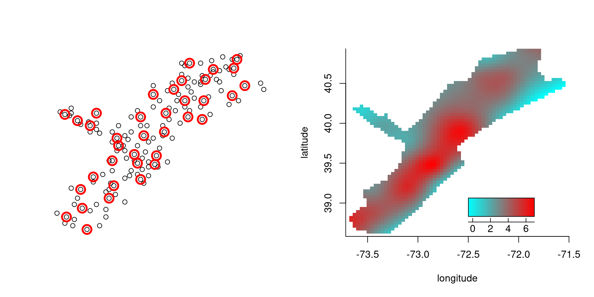
6.2.14 Example: Scallop Catches

Data records location and size of scallop catches off Long Island.

A bivariate penalized spline fit is computed by

data(scallop)
attach(scallop)
log.catch <- log(tot.catch + 1)
out <- capture.output(fit <- spm(log.catch ~ f(longitude, latitude)))
summary(fit)
## 
## 
## Summary for non-linear components:
## 
##                          df   spar knots
## f(longitude,latitude) 25.12 0.2904    37

Default knot locations are determined using clara.

Knot locations and fit:

A fit using mgcv would use

scallop.gam <- gam(log.catch ~ s(longitude, latitude), data = scallop)
summary(scallop.gam)
## 
## Family: gaussian 
## Link function: identity 
## 
## Formula:
## log.catch ~ s(longitude, latitude)
## 
## Parametric coefficients:
##             Estimate Std. Error t value Pr(>|t|)    
## (Intercept)   3.4826     0.1096   31.77   <2e-16 ***
## ---
## Signif. codes:  
## 0 '***' 0.001 '**' 0.01 '*' 0.05 '.' 0.1 ' ' 1
## 
## Approximate significance of smooth terms:
##                         edf Ref.df     F p-value    
## s(longitude,latitude) 26.23  28.53 8.823  <2e-16 ***
## ---
## Signif. codes:  
## 0 '***' 0.001 '**' 0.01 '*' 0.05 '.' 0.1 ' ' 1
## 
## R-sq.(adj) =  0.623   Deviance explained =   69%
## GCV = 2.1793  Scale est. = 1.7784    n = 148

Plot of the fit:

plot(scallop.gam, se = FALSE)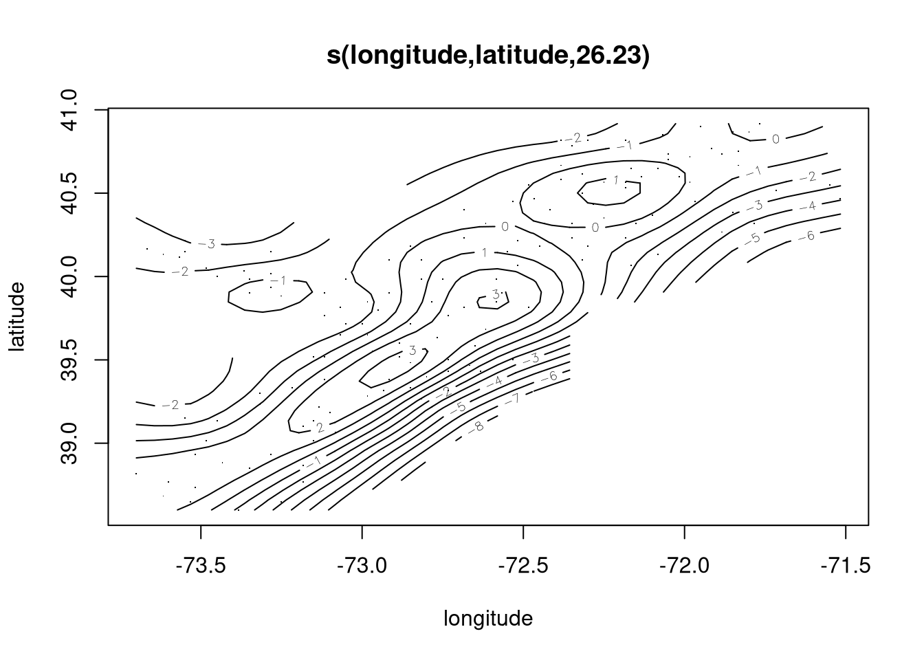

6.2.15 Computational Issues

Algorithms that select the smoothing parameter typically need to compute smooths for many parameter values.

Smoothing splines require solving an $n \times n$ system.

For a single variable the fitting system can be made tri-diagonal.
For thin plate splines of two or more variables the equations are not sparse.

Penalized splines reduce the computational burden by choosing fewer knots, but then need to select knot locations.

Thin plate regression splines (implemented in the mgcv package) use a rank $k$ approximation for a user-specified $k$.

As long as the number of knots or the number of terms $k$ is large enough results are not very sensitive to the particular value of $k$.

Examples are available on line.

\(K(u)\)	Range	Name
\(1/2\)	\|\(u\)\| < 1	Uniform, Boxcar
\(\frac{1}{\sqrt{2\pi}} e^{-u^2/2}\)		Gaussian
1 - \|\(u\)\|	\|\(u\)\| < 1	Triangular
\(\frac{3}{4}(1-u^2)\)	\|\(u\)\| < 1	Epanechnikov
\(\frac{15}{16}(1-u^2)^2\)	\|\(u\)\| < 1	Biweight