 is
is
This section describes a set of tools for computing approximate posterior moments and marginal densities in XLISP-STAT. The definitions needed are in the file bayes.lsp on the distribution disk. This file is not loaded automatically at start up; you should load it now, using the Load item on the File menu or the load command, to carry out the calculations in this section. The material in this section is somewhat more advanced as it assumes you are familiar with the basic concepts of Bayesian inference.
The functions described in this section can be used to compute first and second order approximations to posterior moments and saddlepoint-like approximations to one dimensional marginal posterior densities. The approximations, based primarily on the results in [18,19,20], assume the posterior density is smooth and dominated by a single mode. The implementation is experimental and may change in a number of ways in the near future.
Let's start with a simple example, a data set used to study the relation between survival time (in weeks) of leukemia patients and white blood cell count recorded for the patients at their entry into the study [9, Example U,]. The data consists of two groups of patients classified as AG positive and AG negative. The data for the 17 AG positive patients, contained in the file leukemia.lsp in the Data folder on the distribution disk, can be entered as
(def wbc-pos (list 2300 750 4300 2600 6000 10500 10000 17000 5400 7000
                   9400 32000 35000 100000 100000 52000 100000))
(def times-pos (list 65 156 100 134 16 108 121 4 39 143 56 26 22 1 1 5 65))
A high white blood cell count indicates a more serious stage of the
disease and thus a lower chance of survival.
A model often used for this data assumes the survival times are
exponentially distributed with a mean that is log linear in the
logarithm of the white blood cell count. For convenience I will scale
the white blood cell counts by 10000. That is, the mean survival time
for a patient with white blood cell count  is
is

with  . The log likelihood function is thus
given by

with  representing the survival times. After computing the
transformed WBC variable as
(def transformed-wbc-pos (- (log wbc-pos) (log 10000)))the log likelihood can be computed using the function
(defun llik-pos (theta)
  (let* ((x transformed-wbc-pos)
         (y times-pos)
         (theta0 (select theta 0))
         (theta1 (select theta 1))
         (t1x (* theta1 x)))
    (- (sum t1x)
       (* (length x) (log theta0))
       (/ (sum (* y (exp t1x)))
          theta0))))
I will look at this problem using a vague, improper prior distribution
that is constant over the range  ; thus the log
posterior density is equal to the log likelihood constructed above, up
to an additive constant. The first step is to construct a Bayes model
object using the function bayes-model . This
function takes a function for computing the log posterior density and
an initial guess for the posterior mode, computes the posterior mode
by an iterative method starting with the initial guess, prints a short
summary of the information in the posterior distribution, and returns
a model object. We can use the function llik-pos to compute
the log posterior density, so all we need is an initial estimate for
the posterior mode. Since the model we are using assumes a linear
relationship between the logarithm of the mean survival time and the
transformed WBC variable a linear regression of the logarithms of
the survival times on
transformed-wbc-pos should provide reasonable estimates. The
linear regression gives
> (regression-model transformed-wbc-pos (log times-pos))

Least Squares Estimates:

Constant                  3.54234   (0.302699)
Variable 0              -0.817801   (0.214047)

R Squared:                 0.4932
Sigma hat:                1.23274
Number of cases:               17
Degrees of freedom:            15
so reasonable initial estimates of the mode are
 and
and  . Now we can use these estimates
in the
bayes-model function:
> (def lk (bayes-model #'llik-pos (list (exp 3.5) .8)))
maximizing...
Iteration 0.
Criterion value = -90.8662
Iteration 1.
Criterion value = -85.4065
Iteration 2.
Criterion value = -84.0944
Iteration 3.
Criterion value = -83.8882
Iteration 4.
Criterion value = -83.8774
Iteration 5.
Criterion value = -83.8774
Iteration 6.
Criterion value = -83.8774
Reason for termination: gradient size is less than gradient tolerance.


First Order Approximations to Posterior Moments:

Parameter 0                56.8489 (13.9713)
Parameter 1               0.481829 (0.179694)

#<Object: 1565592, prototype = BAYES-MODEL-PROTO>
>
It is possible to suppress the summary information by supplying NIL as the value of the :print keyword argument.
The summary printed by bayes-model gives first order approximations to the posterior means and standard deviations of the parameters. That is, the means are approximated by the elements of the posterior mode and the standard deviations by the square roots of the diagonal elements of the inverse of the negative Hessian matrix of the log posterior at the mode. These approximations can also be obtained from the model by sending it the :1stmoments message:
> (send lk :1stmoments)
((56.8489 0.481829) (13.9713 0.179694))
The result is a list of two lists, the means and the standard deviations. A slower but more accurate second order approximation is available as well. It can be obtained using the message :moments:
> (send lk :moments)
((65.3085 0.485295) (17.158 0.186587))
Both these messages allow you to compute moments for individual parameters or groups of parameters by specifying an individual parameter index or a list of indices:
> (send lk :moments 0)
((65.3085) (17.158))
> (send lk :moments (list 0 1))
((65.3085 0.485295) (17.158 0.186587))
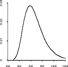
The first and second order approximations to the moments of
 are somewhat different; in particular the mean appears to
be somewhat larger than the mode. This suggests that the posterior
distribution of this parameter is skewed to the right. We can confirm
this by looking at a plot of the approximate marginal posterior
density. The message :margin1 takes a parameter index, and a
sequence of points at which to evaluate the density and returns as its
value a list of the supplied sequence and the approximate density
values at these points. This list can be given to plot-lines
to produce a plot of the marginal density:
> (plot-lines (send lk :margin1 0 (rseq 30 120 30)))
#<Object: 1623804, prototype = SCATTERPLOT-PROTO>
The result is shown in Figure 20 and does indeed show some skewness to the right.

Figure 20: Plot of marginal posterior density for  .
.
In addition to examining individual parameters it is also possible to
look at the posterior distribution of smooth functions of the
parameters.![]() For example, you might want to ask what information the
data contains about the probability of a patient with WBC = 50000
surviving a year or more. This probability is given by
For example, you might want to ask what information the
data contains about the probability of a patient with WBC = 50000
surviving a year or more. This probability is given by

with

and  , and can be computed by the function
(defun lk-sprob (theta)
  (let* ((time 52.0)
         (x (log 5))
         (mu (* (select theta 0) (exp (- (* (select theta 1) x))))))
    (exp (- (/ time mu)))))
This function can be given to the :1stmoments,
:moments and :margin1 methods to approximate the
posterior moments and marginal posterior density of this function. For
the moments the results are
> (send lk :1stmoments #'lk-sprob)
((0.137189) (0.0948248))
> (send lk :moments #'lk-sprob)
((0.184275) (0.111182))
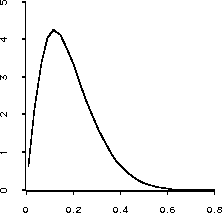
with the difference again suggesting some positive skewness, and the marginal density produced by the expression
(plot-lines (send lk :margin1 #'lk-sprob (rseq .01 .8 30)))is shown in Figure 21. Based on this picture the data suggests that this survival probability is almost certainly below 0.5, but it is difficult to make a more precise statement than that.

Figure 21: Plot of marginal posterior density of the one year survival
probability of a patient with WBC = 50000.
The functions described in this section are based on the optimization code described in the previous section. By default derivatives are computed numerically. If you can compute derivatives yourself you can have your log posterior function return a list of the function value and the gradient or a list of the function value, the gradient and the Hessian matrix.