XLISP-STAT allows the construction of nonlinear, normal regression models. The present implementation is experimental. The definitions needed for nonlinear regression are in the file nonlin.lsp on the distribution disk. This file is not loaded automatically at start up; you should load it now, using the Load item on the File menu or the load command, to carry out the calculations in this section.
As an example, Bates and Watts [1, A1.3,] describe an experiment on the relation between the velocity of an enzymatic reaction, y, and the substrate concentration, x. The data for an experiment in which the enzyme was treated with Puromycin are given by
(def x1 (list 0.02 0.02 0.06 0.06 .11 .11 .22 .22 .56 .56 1.1 1.1))
(def y1 (list 76 47 97 107 123 139 159 152 191 201 207 200))
The Michaelis-Menten function

often provides a good model for the dependence of velocity on substrate concentration. Assuming the Michaelis-Menten function as the mean velocity at a given concentration level the function f1 defined by
(defun f1 (b) (/ (* (select b 0) x1) (+ (select b 1) x1)))computes the list of mean response values at the points in x1 for a parameter list b. Using these definitions, which are contained in the file puromycin.lsp in the Data folder of the distribution disk, we can construct a nonlinear regression model using the nreg-model function.
First we need initial estimates for the two model parameters.
Examining the expression for the Michaelis-Menten model shows that as
x increases the function approaches an asymptote,  . The
second parameter,
  , can be interpreted as the value of x
at which the function has reached half its asymptotic value. Using
these interpretations for the parameters and a plot constructed by the
expression
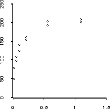
(plot-points x1 y1)shown in Figure 19 we can read off reasonable initial estimates of 200 for
 and 0.1 for
  . The
nreg-model function takes the mean function, the response vector
and an initial estimate of the parameters, computes more accurate
estimates using an iterative algorithm starting from the initial
guess, and prints a summary of the results. It returns a nonlinear
regression model object:

Figure 19: Plot of reaction velocity against substrate concentration for
Puromycin experiment.
> (def puromycin (nreg-model #'f1 y1 (list 200 .1)))
Residual sum of squares:    7964.19
Residual sum of squares:    1593.16
Residual sum of squares:    1201.03
Residual sum of squares:    1195.51
Residual sum of squares:    1195.45
Residual sum of squares:    1195.45
Residual sum of squares:    1195.45
Residual sum of squares:    1195.45

Least Squares Estimates:

Parameter 0               212.684   (6.94715)
Parameter 1             0.0641213   (0.00828094)

R Squared:               0.961261
Sigma hat:                10.9337
Number of cases:               12
Degrees of freedom:            10

PUROMYCIN
>
The function nreg-model also takes several keyword arguments, including :epsilon to specify a convergence criterion and :count-limit, a limit on the number of iterations. By default these values are .0001 and 20, respectively. The algorithm for fitting the model is a simple Gauss-Newton algorithm with backtracking; derivatives are computed numerically.
To see how you can analyze the model further you can send puromycin the :help message. The result is very similar to the help information for a linear regression model. The reason is simple: nonlinear regression models have been implemented as objects, with the nonlinear regression model prototype nreg-model-proto inheriting from the linear regression model prototype. The internal data, the method for computing estimates, and the method of computing fitted values have been modified for nonlinear models, but the other methods remain unchanged. Once the model has been fit the Jacobian of the mean function at the estimated parameter values is used as the X matrix. In terms of this definition most of the methods for linear regression, such as the methods :coef-standard-errors and :leverages, still make sense, at least as first order asymptotic approximations.
In addition to the messages for linear regression models a nonlinear regression model can respond to the messages
:COUNT-LIMIT
:EPSILON
:MEAN-FUNCTION
:NEW-INITIAL-GUESS
:PARAMETER-NAMES
:THETA-HAT
:VERBOSE