Advanced Calculus using Mathematica
Advanced Calculus using Mathematica: NoteBook Edition is a complete text on calculus of several variables written in Mathematica NoteBooks.
Parametric 1D: Procedure 9.6.1
A regular parameterization gives a direction or orientation to the curve from the starting point X[a] in the direction of ![]() to X[b].
to X[b].
Figure 9.6.2 shows the full-scale figure on the left and a view magnified by 1/δt on the right. After magnification the red error measures ε. When δt≈0 is small, the magnified error ε is small and the magnified displacement from X[t] to X[t+δt] appears to be the same as the linear (in δt) displacement ![]() .
.
Notice that this magnified view depends on the “smooth parameterization” (or “regularity”) condition that ![]() because otherwise magnification by 1/δt does not reveal the vector
because otherwise magnification by 1/δt does not reveal the vector ![]() from the approximation
from the approximation
![]()
The Theorem on Smooth Formulas 3.3.1 is easy to apply, simply verify that the formulas x[t], y[t], z[t], ![]() ,
, ![]() ,
, ![]() are valid in an interval about t to prove smoothness of the functions. Smoothness of the curve requires the additional condition
are valid in an interval about t to prove smoothness of the functions. Smoothness of the curve requires the additional condition ![]() . It boils down to: compute and check that your computation makes sense.
. It boils down to: compute and check that your computation makes sense.
Procedure 9.6.1: Finding the Parametric Tangent Line
Suppose  is smooth in a neighborhood of a particular fixed t and
 ![]() . To find the equation of the line tangent to the parametric curve X[t] at t do the following steps:
. To find the equation of the line tangent to the parametric curve X[t] at t do the following steps:
1. Compute the general symbolic derivatives ![]() , y'[t],
, y'[t], ![]() and differential,
and differential,
![]() or
or 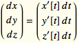
(the symbolic derivatives are functions of t)
2. Calculate the specific values of the derivatives at the particular t, ![]() ,
, ![]() ,
, ![]() , and write the specific total differential at this point:
, and write the specific total differential at this point:
d X=Vd t or 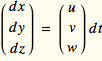
The coefficient V is a specific vector or u, v, and w are specific numbers. This is one vector tangent to the curve at t, provided it is not zero.
3. (Optional) If you want the equation of the tangent plane in (x,y,z)-coordinates, say ![]() ,
, ![]() ,
, ![]() is your particular point of tangency and
is your particular point of tangency and ![]() ,
, ![]() ,
, ![]() is your particular velocity. The local (d x,d y,d z)-coordinates are related to (x,y,z)-coordinates by
is your particular velocity. The local (d x,d y,d z)-coordinates are related to (x,y,z)-coordinates by ![]() ,
, ![]() , and
, and ![]() , so replace d x, d y, and d z with
, so replace d x, d y, and d z with ![]() ,
, ![]() , and
, and ![]() , obtaining the equation:
, obtaining the equation:
![]() or
or ![]() or
or 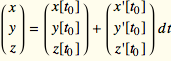
This procedure is programmed in Section 9.5.
You can plot the tangent line using the equation in local coordinates (d x,d y,d z) centered on the curve at the particular X[t] from Step 2. The graph of this equation is a parametric line through the (d x,d y,d z)-origin centered at the point X[t].
The result of Step 3 is a parametric line through ![]() with constant velocity
with constant velocity ![]() and parameter d t. Notice that to correctly evaluate this final expression, you need to perform steps (1), (2), and (3) in that order.
and parameter d t. Notice that to correctly evaluate this final expression, you need to perform steps (1), (2), and (3) in that order.
Notice that the procedure breaks down if ![]() because the parametric graph of
because the parametric graph of ![]() is just the point
is just the point ![]() and not a line. We require
and not a line. We require ![]() in order to know that the curve C that X[t] parameterizes is geometrically smooth. (See the non-smooth parametric curve below.) This requirement guarantees that the procedure produces a line and magnification shows that it is tangent.
in order to know that the curve C that X[t] parameterizes is geometrically smooth. (See the non-smooth parametric curve below.) This requirement guarantees that the procedure produces a line and magnification shows that it is tangent.
Find the velocity vector and tangent line to the helix

at the point where t=π/6.
Solution
Step 1. The general symbolic differential is
 or derivative
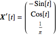
Since all the coordinate functions and all their derivatives are defined everywhere, the function is smooth. Since ![]() , the graph is smooth.
, the graph is smooth.
Step 2. At the particular point where t=π/6,
 or
or 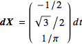
This is the equation of the line through the local ![]() origin with constant velocity
origin with constant velocity  .
.
We place local coordinates at the point ![]() ,
, ![]() ,
, ![]() , draw the constant velocity vector
, draw the constant velocity vector ![]() , and sketch the line through it:
, and sketch the line through it:
Figure: Tangent to a helix