Advanced Calculus using Mathematica
Advanced Calculus using Mathematica: NoteBook Edition is a complete text on calculus of several variables written in Mathematica NoteBooks.
Novel Topics
The text also has a number ot topics that often are not included in a traditonal “calc 3” book or even a stand-alone “Vector Calculus” book.
Constrained differentiation
Partial Derivatives in Thermodynamics ![]()
In thermodynamics there are some important relations between the rates of change of quantities like “internal energy” when variables like pressure or temperature are changed. Some of these rates are directly measurable, while others are not, so we want to relate the indirect ones to the direct ones by mathematical computations. These relationships are a little confusing mathematically because they are “constrained” by an “equation of state.” Mathematically, this means we have a function
U=f[P,V,T] but must maintain P V=k T, for constant k (or P V=n R T, k=n R)
We want to compute the rate of change of U as P changes, holding V fixed, denoted,
![]()
This classical notation typically doesn’t explicitly mention the implicit fact that P V=k T. The quantity T must vary in such a way as to change P, hold V fixed, and maintain P V=k T. If you heat a gas in a fixed volume and can measure the changes in U and P, you have the experimental ![]() .
.
Mathematically, we are computing rates of change of a function of 3 variables, f[P,V,T], when it is restricted to an implicitly defined surface given by P V=k T. Since the implicit constraint P V=k T “determines” one variable in terms of the other two, we know we can only vary two independent quantities at a time, and have the mathematical choices,
![]() :
: ![]()
![]() :
: ![]()
![]() :
: ![]()
Each expression suggests 2 experiments, so the notation is helpful thermodynamically. We have written P V = k T in the solved forms T=T[P,V], etc.
This section shows how to differentiate functions restricted to an implicitly defined manifold, but first begins with the simple case of a function of two variables restricted to an explicit 1D curve.
Second Order Constrained Derivatives
The behavior of second derivatives under constraints is different from the un-constrained Hessian (in Chapter 6). Suppose we have a function f[x,y] subject to a constraint g[x,y]=0. When ∂g/∂y≠0, we can apply the implicit function theorem to locally solve for y=γ[x] ⇔ g[x,y]=0. In effect this makes f[x,y] a function of one variable,
F[x]=f[x,γ[x]]
Constrained differentiation or the Chain Rule on the formula in the implicit function theorem gives
![]() :
: ![]()
Solving the constraint for d y means
![]() or
or ![]()
and substituting in d f gives
![]()
Differentiating the right hand side as a function of both x and y gives:
![]()
Substituting ![]() gives:
gives:
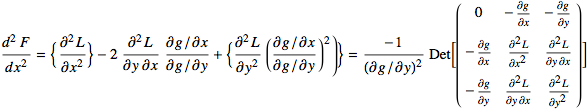
![]()
![]()
If ![]() , and L[x,y]=f[x,y]-λ g[x,y],
, and L[x,y]=f[x,y]-λ g[x,y],
MAX-min
Design parameters
Following is an exercise that uses Mathematica to find eigenvalues.
a) Find the (approximate or floating point numerical) eigenvalues of the quadratic form:
![]()
You may do it by hand if you wish. Show your computer calculation if you use Mathematica or another modern calculator.
b) Does q have a max or min? Justify your answer.
c) If the current design parameters of q are (w,x,y,z)=(1,1,1,1), which direction of CHANGE in (w,x,y,z) will DECREASE q at the fastest rate? If we can only change the vector (1,1,1,1) by 10%, ![]() , what should the new values be?
, what should the new values be?
Bordered Hessians
The regular hessian test for a local extremum does not apply with constraints. The “bordered hessian” is somewhat complicated computationally, but here is a concrete example:
Find the pair of points on the surfaces ![]() and
and ![]() that are closest and farthest.
that are closest and farthest.
We formulate this as find the MAX and min of
![]() subject to
subject to ![]() and
and ![]()
Solving the critical point equations is the hard part. In this example, we use Reduce[.]
Details of finding the real solutions are in the closed cell showing the values.
The real solutions are in this closed cell.
| μ | λ | u | x | v | y | w | z | f |
| -6.05664 | 6.99061 | -0.0852534 | 1.70457 | 0.361587 | -2.16551 | -1.30192 | 3.24866 | 5.50432 |
| -3.45858 | -3.55392 | 0.135644 | 1.58185 | -0.453922 | -2.06713 | 1.21553 | 3.37548 | 3.0593 |
| 6.43099 | -6.10988 | 0.121492 | 2.34635 | -0.575552 | -4.09414 | 1.11732 | 4.53078 | 5.38351 |
| 8.94952 | 9.55424 | -0.112224 | 2.28723 | 0.453669 | -3.99923 | -1.23983 | 4.65812 | 7.76991 |
The bordered hessian:
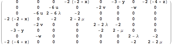
The determinant sequence at the first critical point:
![]()
![]()
![]()
![]()
![]()
![]()
This is a saddle point.
Project on MAX-min: Resonance
Resonance is a peak in vibration as you vary the frequency at which you “shake” a system. For example, many old cars have speeds where they hum loudly, say at 47 mph. Slower, it’s quieter and faster it’s also quieter. We will see this phenomenon in the solution of the linear electrical R-L-C series circuit
![]()
This differential equation expresses Kirchoff’s second law: In a closed circuit the applied voltage is equal to the sum of the voltage drops in the rest of the circuit.
A series R-L-C circuit
Figure 16
Series R-L-C circuit with applied voltage E[t]
Voltage drop due across a resistor of R-ohms due to current i : R i
Voltage drop due across an inductor of L-henries due to a varying current i : ![]()
Voltage drop due across a capacitor of C-farads due to a accumulating current: ![]()
so Kirchoff’s law for a series circuit says:
![]()
The Problem: Find the local maximum amplitude response in terms of the Parameters R, L, C
Implicit Functions
Graphs alone justify use of Mathematica
It is not hard to find the critical points of ![]() (a normal covariance density function), but it is difficult to graph this function by hand. Mathematica makes it easy and even interactive.
(a normal covariance density function), but it is difficult to graph this function by hand. Mathematica makes it easy and even interactive.
Non-elementary Inverses
Most calculus books mention that fact that the integral of the normal probability distribution ![]() is “non-elementary,” that is, can not be expressed in terms of sine, cosine, log and esponential functions.
is “non-elementary,” that is, can not be expressed in terms of sine, cosine, log and esponential functions.
The period of the pendulum is also a non-elementary integral studied in Section 3.7. Linearization of the pendulum is studied there and in Chapter 5. (See below under flows.)
Many arclength integrals are also non-elementary. The arclength of an ellipse corresponds to the distance a planet travels under Kepler's laws and must have occupied much time in trying to find an integral until Louville showed that it is non-elementary 150 years after Newton.
Mathematica can compute these symbolically in terms of its powerful array of (non-elementary) built in functions. The "Gas, Brakes, and Tires" eLab asks students to use Mathematica to find a distance traveled along a "pringles" curve in terms of that non-elementary integral.
Non-elementary functions also arise in the study of inverse functions. For example, ![]() is increasing for x>1/e, so has in inverse in that range. That inverse is non-elementary, see Example 5.0.5, so while the inverse “exists” it can not be written in terms of the high school functions. Mathematica expresses the inverse in terms of the ProductLog function.
is increasing for x>1/e, so has in inverse in that range. That inverse is non-elementary, see Example 5.0.5, so while the inverse “exists” it can not be written in terms of the high school functions. Mathematica expresses the inverse in terms of the ProductLog function.
Flows
Of vector fields
One of the important themes of vector calculus involves computation of rates of flow across boundaries. The actual flows are often not part of beginning courses. Mathematica makes it easy to create animated flows associated with a vector field. See Section 11.3.
Two Advanced Theorems from Chapter 5 On Implicit Functions
Theorem: The “Cauchy” Existence-Uniqueness Theorem with Smooth Dependence on Initial Conditions
Let E be a B-space, a complete normed space. Suppose the function f[X,t] from F×R→E is r-times continuously differentiable on the open set F⊂E. Then the initial value problem ![]() &
& ![]() has a unique solution for some interval of time (-τ,τ). More specifically, there is an open neighborhood V of
has a unique solution for some interval of time (-τ,τ). More specifically, there is an open neighborhood V of ![]() a real τ>0 and a function Φ[X,t]:E×(-τ,τ)→U such that:
a real τ>0 and a function Φ[X,t]:E×(-τ,τ)→U such that:
(1) Φ[X,t] is r-times continuously differentiable
(2) Φ[X,0]=X, for X∈V (the initial condition)
(3) ![]() , for -τ<t<τ and X∈V.
, for -τ<t<τ and X∈V.
It is interesting to observe that the proof of this theorem follows from the Inverse Function Theorem as shown in Chapter 5.
The case of an “autonomous” differential equation where the function f does not depend on time, corresponds to finding “streamlines” of a flow.
If F[X] is a smooth vector field describing the velocity of a fluid on a region, then velocity is also the time derivative, so ![]() when X[t] is a parametic curve, or a single streamline. This is the case of the above theorem when f[X,t]=F[X] does not depend on time. The flow associated with F can be thought of as the function Φ[X,t] that gives the position of points in time along a streamline starting at the point X. We study these equations in Section 11.3 and 11.6.
when X[t] is a parametic curve, or a single streamline. This is the case of the above theorem when f[X,t]=F[X] does not depend on time. The flow associated with F can be thought of as the function Φ[X,t] that gives the position of points in time along a streamline starting at the point X. We study these equations in Section 11.3 and 11.6.
The “infinitesimal microscope” idea also applies to flows as follows.
Theorem: Microscopic Equilibria (F. & M. Diener)
Let f [x, y] and g[x, y] be smooth functions with ![]() . The flow of
. The flow of

under infinite magnification at ![]() appears the same as the flow of its linearization
appears the same as the flow of its linearization
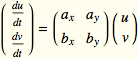 ,
,
![]() ,
, ![]() ,
, ![]() ,
, ![]()
Specifically, if our magnification is 1/δ,for δ≈0, and our solution starts in our view, � � � �� � � � Specifically, if our magnification is 1/δ,forδ0, and our solution starts in our view, � � � �� � � � Specifically, if our magnification is 1/δ,forδ0, and our solution starts in our view, Specifically, if our magnification is 1/δ,forδ0, and our solution starts in our view, Specifically, if our magnification is 1/δ,forδ0, and our solution starts in our view,
![]()
for limited a and b and if (u[t],v[t]) satisfies the linear equation and starts at (u[0],v[0]) = (a, b),then� � � �� � � � Specifically, if our magnification is 1/δ,forδ0, and our solution starts in our view, � � � �� � � � Specifically, if our magnification is 1/δ,forδ0, and our solution starts in our view, Specifically, if our magnification is 1/δ,forδ0, and our solution starts in our view, Specifically, if our magnification is 1/δ,forδ0, and our solution starts in our view,
![]()
where ![]() for all limited t.
for all limited t.
This is a fun and easy theorem - the pictures work even when the eigenvalues of the linear system are zero! where nothing moves in the linear view.
Figure 12.12.7: Microscopic views of a nonlinear flow
Figure 17
Linearizing the Pendulum
A frictionless pendulum on a weightless rigid rod is governed by the equations
 with
with ![]()
where θ is the angle the rod makes from the vertical, g is the gravitational constant in your units, and L is the length of the pendulum. (See Projects for Calclulus: The Language of Change, by Keith Stroyan, Project 46.) These equations have an equilibrium at ![]() . At this point, the linearized equations are
. At this point, the linearized equations are
 with solution
 ![]() when
when ![]() (in other words if the pendulum is released from rest at angle α.)
(in other words if the pendulum is released from rest at angle α.)
![]()
![]()
The flow of the linear equation is rotation around circles at angular frequency ![]() . By Diener’s theorem above, the angular frequency of the nonlinear pendulum is infinitely close to this value when the oscillations are infinitesimal, α≈0. This result can also be obtained from the exact formula for the period of the nonlinear pendulum in Exercise 3.7.6.
. By Diener’s theorem above, the angular frequency of the nonlinear pendulum is infinitely close to this value when the oscillations are infinitesimal, α≈0. This result can also be obtained from the exact formula for the period of the nonlinear pendulum in Exercise 3.7.6.
The pendulum is viewed as motion constrained to a circle in Exercise 16.2.6.
Osculating Circle and Sphere
The osculating circle is tangent to the curve at a given point and has radius r=1/κ, as in the case where the curve is a circle (with constant curvature κ=1/r as shown in the Example 9.8.1.) Since the Kurvature vector is perpendicular to the curve (by Theorem 9.8.2), the center of the osculating circle lies on the line through X[t] in the direction of K[t] at a distance 1/κ[t] from the point of tangency.
Figure: Moving the Osculating Circle along ![]()
Figure 18
The osculating circle is also a limit of the circle through three points on a curve in the limit as the three points tend together.
Figure: A Circle through three points of ![]()
Figure 19
If we take four nearby points on a curve in 3D and fit a sphere, the limit is the “Osculating Sphere” that incorporates curvature and torsion geometrically.
Figure: Moving the Osculating Sphere
Figure 20
Surface curvature
Extending the 2D curve idea above, we consider the image of a portion of our surface mapped onto the unit sphere by the “Gauss map” Γ shown in Figure 16.1.3.
Figure: Gauss Map Images at Low and High Curvature
Figure 21
Divergence and Curl as the symmetric and antisymmetric decompositon of the total derivative
Microscopic Divergence and “Curl” in 2D
See the microscopic divergence and curl sections above where we show that local linearity plus Duhamel’s Principle gives Green’s Theorem.
Microscopic Divergence and Curl in 3D
See the microscopic divergence and curl sections above where we show that local linearity plus Duhamel’s Principle gives Green’s Theorem.
Section 18.6 shows how to “see” the divergence and curl as the symmetric and antisymmetric decomposition of the derivative of a vector field.
Vector Potentials
Functional dependence
When the total differential does not have full rank some component functions are functions of others. Section 5.6 explains this situation and applies it to the local problem of finding a vector field whose curl equals a given vector field with zero divergence.
An Integral Formula for the Vector Potential
Section 18.4 gives a local integral formula for the vector potential. The next topic considers some special cases of the global question.
Handles & bubbles
Theorem 14.4.3 shows that if the divergence of a vector field is zero, then there is a local “vector potential.” (In terms of 2-forms, if a 2-form Ω has d∧Ω=0, then locally there is a 1- form ω with d∧ω=Ω.) This section gives examples that show that the the ability to find a global “antiderivative” of this kind depends on the tolology ot the domain.
In Section 19.4 we showed that
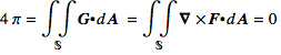
![]() , has zero divergence, ∇•G=0, except at the origin where it is undefined. (Also see Example 18.4.5)
, has zero divergence, ∇•G=0, except at the origin where it is undefined. (Also see Example 18.4.5)
Let S be any closed surface not containing the origin that is the boundary of a compact solid domain D. Then
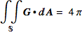 if the origin lies in the interior of D
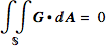 if the origin does not lie in the interior of D
Even though the divergence of G is zero, G can not be the curl of any vector field on 3-space less the origin. Stokes’ Theorem on a gives
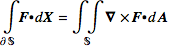
but if the boundary is zero because the surface is closed, the left side is zero (see Exercise 19.2.8.) Thus we can not have
This failure to be able to antidifferentiate G “measures” a bubble in the domain where the origin was removed.
Theorem 13.13.1: A special case of second homology
Suppose F is a smooth vector field on 3-space less the origin and ∇•F[X]=0 for all X≠0. Then there is a vector field P[X] smooth except possibly at the origin so that F[X]=φ G[X]+∇×P[X] where 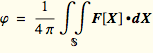 for the unit sphere S centered at the origin.
A Vector Field with Invariant Flux from Tori
See Example 17.4.4 where we give toroidal coordinates and Exericse 17.5.3 where we give derivatives in these coordinates. Also see Example 19.3.7 where we look at path integrals in this space.
The vector field given next has a basic relation to the surface topology inside the donut space.
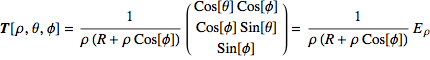
Exericse 17.5.3 shows that ∇• T = 0.
Let S be any closed surface not containing the circle ![]() that is the boundary of a compact solid domain D. Then
that is the boundary of a compact solid domain D. Then
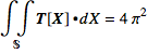 if the C lies in the interior of D
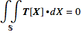 if the C does not lie in the interior of D
Theorem 14.4.3 shows that if the divergence of a vector field is zero, then there is a local “vector potential,” but even though the divergence of T is zero, T can not be the curl of any vector field on 3-space less the origin. Stokes’ Theorem on a “closed” surface gives integral zero, just as in the inverse square law example above.
This failure to be able to antidifferentiate T “measures” a handle in the domain where the circle was removed.
Theorem 14.14.2: A special case of second homology
Suppose F is a smooth vector field on a donut 0<ρ<R and ∇•F[X]=0 for all X∉ C. Then there is a vector field P[X] smooth except possibly on C so that F[X]=φ T[X]+∇×P[X] where 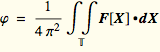 for the unit torus T centered on C.
We can state the local “Curl Test” and the “Divergence Test” in differential form notation, where the result is known as the “Poincare’s Lemma.” The condition ![]() for a 1-form means the coefficients form a vector field with zero curl. The condition
for a 1-form means the coefficients form a vector field with zero curl. The condition ![]() for a 2-form means the coefficients form a vector field with zero divergence.
for a 2-form means the coefficients form a vector field with zero divergence.
Heat equation
Section 15.15: The Heat Equation ![]()
In this section we show how Gauss' Divergence Theorem gives rise to the “heat equation.” An eLab has you solve the heat equation in a special case.
Derivation of the Heat Equation for a homogeneous isotropic body
Well-posed Problems for the Heat Equation
Steady state temperature distributions and Laplace's Equation