Advanced Calculus using Mathematica
Advanced Calculus using Mathematica: NoteBook Edition is a complete text on calculus of several variables written in Mathematica NoteBooks.
Computer work
Most of the day-to-day work in our courses is traditional paper and pencil work. The text mostly looks like an on-screen old-fashioned math book. For example, the various cases of the tangent procedure above are excerpts of the text (transferred to a web page.) We start student computing with some very simple programs like solutions to many exercises.
About once a week we have an “eExercise” such as graphing a surface z=f[x,y] and its tangent plane. In these basic programming assignments, we strive to show the students how the textbook material written as Mathematica commands gives the solution. We find it best if the instructor helps students type some of the basic programs, even though there are examples in the eSections of the text that they could copy, paste, and modify. Mathematica looks very similar to conventional math, but programming syntax gives no partial credit - you have to have all the commas and curly ques in the right places. At the end of this eExercise students should have a clearer idea of the algorithm that produces the tangent plane.
We also assign a few more difficult eExercises. These build on one of the students earlier basic programs, but add a mathematical problem. Following are some examples:
Steepest Tangent
The gradient points in the direction of steepest ascent, but suppose you want to add a tangent vector pointing up hill to your program that shows an explicit graph z=f[x,y] with its tangent plane. The gradient ![]() is only 2D, although it points in the right direction in (x.y)-space. Students are asked to develop a formula for the steepest tangent in 3D and add it to their program.
is only 2D, although it points in the right direction in (x.y)-space. Students are asked to develop a formula for the steepest tangent in 3D and add it to their program.
Moment of Inertia
Construct Physical Objects
Make the following shapes out of a thin flat uniform density material in the dimensions shown. It would be helpful if they all had the same total mass. For example, the rectangle has twice the area of the triangle, so making the triangle double thickness would give it the same mass. (Dumpster diving for cardboard will work. You don’t need to spend a lot on materials.)
Center of Gravity
Calculate the center of gravity of each shape, drill a hole in each at that point and suspend it from a thin string through the hole.
Moment of Inertia
Calculate the moment of inertia of each shape about the origin as shown in the figure above. (You can use polar coordinates for the half-disk, but be careful.)
Equal Total Mass Comparison
Assuming the three shapes have the same total mass (because they are different thicknesses or densities), which has the largest moment of inertia, which is second, which is third? (You can either set up your integrals with the thickness and mass density included or use the radius of gyration from Exercise 8.3.12 or Exercise 13.2.8. Again, use Mathematica for the calculations if you wish.)
Physics of Moments
Devise a physical experiment to show which object has the largest moment of inertia, which is next and which is smallest. This comparison should assume that the total mass of all the objects is the same. If your physical objects are not the same mass (and that’s OK), show how to calculate the comparison with same mass from your experiment.
If you develop a little physical “intuition” about the sum defining moment of inertia, you should be able to guess the largest fairly easily. The next two take some computation. The tricky part is the “same mass” assumption.
Gas, Brakes, & Tires
Let position be X[t], velocity be V[t], speed be v[t], and acceleration be A[t].
a) Make a program that animates the motion of a point that moves in all 3 dimensions of space. Show its changing position vector, its velocity vector at the tip of the position vector, and its acceleration vector at the tip of the velocity vector. (There is a sample animation in eSection 9.5. Velocity and acceleration are easily defined in Mathematica, see Section 10.1.) Your animation should look like:
b) Give a specific time on your motion when the SPEED is increasing, a time when speed is decreasing, and a time when speed is not changing, but acceleration is not zero. Justify your answers.
HINT: See Exercise 10.2.1 and inClass Activity 10.1 and plot your speed function:

c) Suppose your animation represents a driver racing around a curving road. When the angle between the velocity and acceleration vectors is acute is the driver stepping on the gas or the brakes?
d) At the time on your animation where speed is not changing, but acceleration is not zero, what force is providing the acceleration?
e) Calculate the distance along your curve from the position at t=0 to each of the points of part (b).
Weierstrass’ Wild Wiggles: A nowhere differentiable function
Microscopic views of W[x]
Write a program to plot ![]() for c-1/M≤x≤c+1/M, W[c]-1/M≤y≤W[c]+1/M, to within one pixel. Use the smallest n so that the approximation
for c-1/M≤x≤c+1/M, W[c]-1/M≤y≤W[c]+1/M, to within one pixel. Use the smallest n so that the approximation ![]() is guaranteed to have one pixel accuracy for a given M and c. (We should be able to change M and c in your program and still have it plot to within one pixel.)
is guaranteed to have one pixel accuracy for a given M and c. (We should be able to change M and c in your program and still have it plot to within one pixel.)
a) Your formula for n=? (A function of M. Help follows below. This is the MAIN part of the assignment. A fixed n in your program receives ZERO credit.)
b) Use your program to graph W[x] centered at x-center c=0.5 at magnification 1 and compare to the graph in the background section below. Then zoom in on the graph at magnification 10 and 100 at the x-centers c=0.3,0.4,0.5
c) Differentiate the series ![]() term-by-term. Does this series converge? Plot several terms of the series, say 4 terms, then 8 terms, then 16 or a Manipulate program with variable n.
term-by-term. Does this series converge? Plot several terms of the series, say 4 terms, then 8 terms, then 16 or a Manipulate program with variable n.
 &
& 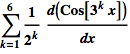
Figure 15