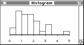
Figure 1: Histogram of precipitation levels.
Devore and Peck [11, page 54, Table 10,] give precipitation levels recorded during the month of March in the Minneapolis - St. Paul area over a 30 year period. Let's enter these data into XLISP-STAT with the name precipitation:
> (def precipitation
       (list .77 1.74 .81 1.20 1.95 1.20 .47 1.43 3.37 2.20 3.30
             3.09 1.51 2.10 .52 1.62 1.31 .32 .59 .81 2.81 1.87
             1.18 1.35 4.75 2.48 .96 1.89 .90 2.05))
PRECIPITATION
>
In typing this expression I have hit the return and
tab keys a few times in order to make the typed expression easier
to read. The tab key indents the next line to a reasonable point to
make the expression more readable.
The histogram and boxplot functions can be used to obtain graphical representations of this data set:
> (histogram precipitation)
#<Object: 3564170, prototype = HISTOGRAM-PROTO>
> (boxplot precipitation)
#<Object: 3423466, prototype = SCATTERPLOT-PROTO>
>

Figure 1: Histogram of precipitation levels.
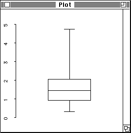
Each of these commands should cause a window with the appropriate graph to appear on your screen. The windows should look something like Figures 1 and 2.

Figure 2: Boxplot of precipitation levels.
Note that as each graph appears it becomes the active window. To get XLISP-STAT to accept further commands you have to click on the XLISP-STAT listener window. You will have to click on the listener window between the two commands shown here.
The two functions return results that are printed something like this:
#<Object: 3564170, prototype = HISTOGRAM-PROTO>These result will be used later to identify the window containing the plot. For the moment you can ignore them.
When you have several plot windows open you might want to close the listener window so you can rearrange the plots more easily. You can do this by clicking in the listener window's close box. You can later re-open the listener window by selecting the Show XLISP-STAT item on the Command menu.
Here are some numerical summaries:
> (mean precipitation)
1.685
> (median precipitation)
1.47
> (standard-deviation precipitation)
1.0157
> (interquartile-range precipitation)
1.145
>
The distribution of this data set is somewhat skewed to the right. Notice the separation between the mean and the median. You might want to try a few simple transformations to see if you can symmetrize the data. Square root and log transformations can be computed using the expressions
(sqrt precipitation)and
(log precipitation).You should look at plots of the data to see if these transformations do indeed lead to a more symmetric shape. The means and medians of the transformed data are
> (mean (sqrt precipitation))
1.243006
> (median (sqrt precipitation))
1.212323
> (mean (log precipitation))
0.3405517
> (median (log precipitation))
0.384892
>
The boxplot function can also be used to produce parallel boxplots of two or more samples. It will do so if it is given a list of lists as its argument instead of a single list. As an example, let's use this function to compare serum total cholesterol values for samples of rural and urban Guatemalans (Devore and Peck [11, page 19, Example 3,]):
> (def urban (list 184 196 217 284 184 236 189 206 179 170 205 190
                   204 330 217 242 222 242 249 241))
URBAN
> (def rural (list 166 146 144 204 158 143 158 180 223 194 194 175
                   171 155 143 145 131 181 148 144 220 129))
RURAL
>
The parallel boxplot is obtained by
> (boxplot (list urban rural))
#<Object: 3423466, prototype = SCATTERPLOT-PROTO>
>
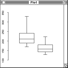
and is shown in Figure 3; the urban group is on the left.

Figure 3: Parallel box plots of cholesterol levels for urban and
rural guatemalans.