Assignment 4
Guidelines
You will submit your homework as an R Markdown (.Rmd) file by committing to your git repository and pushing to GitLab. We will knit this file to produce the .html output file (you do not need to submit the .html, but you should make sure that it can be produced successfully).
We will review both your .Rmd file and the .html file. To receive full credit:
You must submit your
.Rmdfile on time. It must be named exactly as specified, and it must knit without errors to produce a.htmlfile.The
.htmlfile should read as a well written report, with all results and graphs supported by text explaining what they are and, when appropriate, what conclusions can be drawn. Your report should not contain any extraneous material, such as leftovers from a template.The R code in your
.Rmdfile must be clear, readable, and follow the coding standards.The text in your
.Rmdfile must be readable and use R markdown properly, as shown in the class template file.
Create a new folder called HW4 in your repository. Use exactly this spelling with upper case letters. You can do this in the RStudio IDE, with R’s dir.create function, or using a shell.
In this folder, create a new Rmarkdown file called hw4.Rmd. Again use exactly this spelling. RStudio will give you a template, or you can use the one available here. Commit your new file to your repository. (If you are using git in a shell you will need to use git add before git commit).
In this file present your answers to the following problems. Your presentation should follow the pattern and guidelines in the class template file.
1. Evaluate a Visualization
A blog post shows this visualization of donations for research on several diseases and the number of deaths attributed to these diseases:
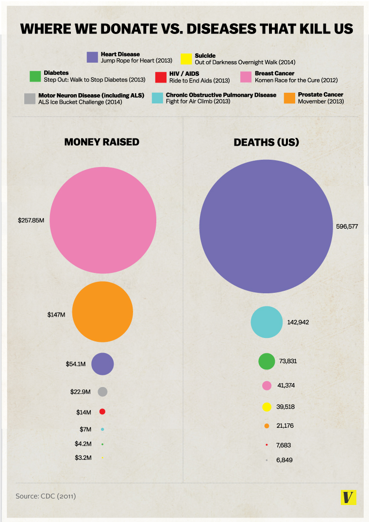
The image is originally from an article at Vox.
The chart now on the Vox site is different; comment on the key change.
Describe the items, attributes, marks, channels, and mappings used in the visualization. Comment on how well the strength of the channels used match the importance of the attributes displayed.
Can you suggest alternatives that might improve on this visualiation in some respects?
The data are available at https://stat.uiowa.edu/~luke/data/dfunds.csv.
2. EPA Fuel Economy Data
The mpg data set provided in the ggplot2 package is rather old: the newest model is from 2008. Newer data is available from the EPA. A compressed CSV file for the years 1984-2024 is available locally and can be downloaded and read in with
library(readr)
if (! file.exists("vehicles.csv.zip"))
    download.file("http://www.stat.uiowa.edu/~luke/data/vehicles.csv.zip",
                  "vehicles.csv.zip")
newmpg <- read_csv("vehicles.csv.zip", guess_max = 100000)
Please do not commit the vehicles.csv.zip file to your repository as it is quite large. Instead, include code in your .Rmd document that downloads the file if necessary.
The data set contains over 80 variables. Read the documentation for the data and identify the variable that specifies the primary fuel type (the fl variable in the mpg data set). Also identify the variables that correspond to the variables hwy, cyl, and displ in the mpg data set.
Using the count function from package dplyr find the number of vehicles for each primary fuel type and present the counts as a nicely formatted table.
Also present the counts as a bar chart. You can do this by using the counts with geom_col or by using geom_bar on the raw data; the default stat for geom_bar will compute the counts for you.
Comment on any interesting features you see in the bar chart.
3. Fuel Type Over the Years
Along the lines of the election data charts in the the notes, create a filled bar chart with one bar for each model year from 1984 through 2024, the complete model years, showing the distribution of primary fuel type within model years. Comment on any interesting features you see.
4. Highway Fuel Economy Over the Years
Create a strip plot showing highway fuel economy values for each of the years from 2000 through 2024. Experiment with the use of jittering and adjusting point size and alpha level to find an effective visualization. Comment on any interesting features you see.
Create an HTML File and Commit Your Work
You can create an HTML file in RStudio using the Knit tab on the editor window. You can also use the R command
rmarkdown::render("hw4.Rmd")with your working directory set to HW4.
Commit your changes to your hw4.Rmd file to your local git repository. You do not heed to commit your HTML file.
Submit your work by pushing your local repository changes to your remote repository on the UI GitLab site. After doing this, it is a good idea to check your repository on the UI GitLab site to make sure everything has been submitted successfully