Data Technology Notes

University of Iowa

College of Liberal Arts and Sciences

Data Technologies
Data Import
Wrangling the Unemployment Data
Refugee Arrival Data
Gapminder Childhood Mortality Data

Data Technologies

Class and homework examples often start with a nice, clean, rectangular data set.

Once you have a source for your data, data technologies are the tools you need to get your data to that point.

The process of applying these tools is sometimes called data wrangling.

The main steps are usually

importing the data;
cleaning the data;
merging information from several sources;
transforming to specialized data types
reshaping the data.

We have seen many of these steps already.

Data Import

Your data may be available in a number of different forms, such as:

as a CSV file;
another form of text file;
a spread sheet;
a table on a web page;
from a web service;
in a SQL data base
in some other type of data base or file format.

We have seen several examples of importing CSV files.

CSV files are often fairly easy to deal with.
They are typically meant for data import rather than human reading.
Spread sheet programs typically provide a mechanism for exporting data in CSV form.
Some issues that you need to look for:
- identifying column names;
- identifing row names;
- use of a semicolon separator (common in Europe).

Unemployment data from the Local Area Unemployment Statistics (LAUS) page ofthe Bureau of Labor Statistics is an example of a structured text file not in CSV format.

These files usually have enough structure for automated import.
Often they have features designed for a human reader that need to be worked around.

Spread sheets are in principle designed for machine computation.

Many spread sheets have features designed for a human reader that need to be worked around.
Exporting (the relevant part of) a spread sheet to CSV is sometimes a good option.
Using a tool that can import directly from the spread sheet is often better: it makes the analysis easier to reproduce and repeat with new data.

Wrangling the Unemployment Data

The unemployment data is available as a text file.

The fields are delimited with a | character and surrounded by white space.
There is a header and a footer that need to be removed.
The counts use a comma to separate thousands.
The column names are awkward.
Some names contain an apostrophe, which can be confused with a quote character.

The base function read.table and the readr function read_table have many options for dealing with these issues.

We can use read.table with:

col.names to specify column names;
skip = 6 to remove the header;
strip_white to remove white space around items
quote = "" to turn off interpreting any character as delimiting a quoted string
fill = TRUE to fill in columns in the footer.

lausURL <- "https://stat.uiowa.edu/~luke/data/laus/laucntycur14-2017.txt"
lausFile <- "laucntycur14-2017.txt"
if (! file.exists(lausFile))
    download.file(lausURL, lausFile)
lausUS <- read.table(lausFile,
                     col.names = c("LAUSAreaCode", "State", "County",
                                   "Title", "Period",
                                   "LaborForce", "Employed",
                                   "Unemployed", "UnempRate"),
                     quote = "", sep = "|", skip = 6, strip.white = TRUE,
                     fill = TRUE)
head(lausUS)
##      LAUSAreaCode State County              Title Period LaborForce Employed
## 1 CN0100100000000     1      1 Autauga County, AL Nov-16     25,809   24,518
## 2 CN0100300000000     1      3 Baldwin County, AL Nov-16     89,507   84,817
## 3 CN0100500000000     1      5 Barbour County, AL Nov-16      8,213    7,546
## 4 CN0100700000000     1      7    Bibb County, AL Nov-16      8,645    8,105
## 5 CN0100900000000     1      9  Blount County, AL Nov-16     24,754   23,481
## 6 CN0101100000000     1     11 Bullock County, AL Nov-16      4,990    4,609
##   Unemployed UnempRate
## 1      1,291       5.0
## 2      4,690       5.2
## 3        667       8.1
## 4        540       6.2
## 5      1,273       5.1
## 6        381       7.6
tail(lausUS)
##                                                                                                                                 LAUSAreaCode
## 45066                                                                                                                        CN7215300000000
## 45067 --------------------------------------------------------------------------------------------------------------------------------------
## 45068                                                                                                                     (p) = preliminary.
## 45069                                                                                            Dash indicates that data are not available.
## 45070                                                                                                                      SOURCE: BLS, LAUS
## 45071                                                                                                                       February 6, 2018
##       State County               Title    Period LaborForce Employed Unemployed
## 45066    72    153 Yauco Municipio, PR Dec-17(p)     10,523    8,892      1,631
## 45067    NA     NA                                                             
## 45068    NA     NA                                                             
## 45069    NA     NA                                                             
## 45070    NA     NA                                                             
## 45071    NA     NA                                                             
##       UnempRate
## 45066      15.5
## 45067          
## 45068          
## 45069          
## 45070          
## 45071

Searching for a sequence of dashes allows the code to drop the footer to work even if the number of rows changes.

footstart <- grep("------", lausUS$LAUSAreaCode)
lausUS <- lausUS[1:(footstart - 1), ]

str show the data types we now have:

str(lausUS)
## 'data.frame':    45066 obs. of  9 variables:
##  $ LAUSAreaCode: chr  "CN0100100000000" "CN0100300000000" "CN0100500000000" "CN0100700000000" ...
##  $ State       : int  1 1 1 1 1 1 1 1 1 1 ...
##  $ County      : int  1 3 5 7 9 11 13 15 17 19 ...
##  $ Title       : chr  "Autauga County, AL" "Baldwin County, AL" "Barbour County, AL" "Bibb County, AL" ...
##  $ Period      : chr  "Nov-16" "Nov-16" "Nov-16" "Nov-16" ...
##  $ LaborForce  : chr  "25,809" "89,507" "8,213" "8,645" ...
##  $ Employed    : chr  "24,518" "84,817" "7,546" "8,105" ...
##  $ Unemployed  : chr  "1,291" "4,690" "667" "540" ...
##  $ UnempRate   : chr  "5.0" "5.2" "8.1" "6.2" ...

Convert the counts to numbers by removing the commas and passing to as.numeric:

lausUS <- mutate(lausUS,
                 LaborForce = as.numeric(gsub(",", "", LaborForce)),
                 Employed = as.numeric(gsub(",", "", Employed)),
                 Unemployed = as.numeric(gsub(",", "", Unemployed)))
## Warning: There were 3 warnings in `mutate()`.
## The first warning was:
## ℹ In argument: `LaborForce = as.numeric(gsub(",", "", LaborForce))`.
## Caused by warning:
## ! NAs introduced by coercion
## ℹ Run `dplyr::last_dplyr_warnings()` to see the 2 remaining warnings.

The expression

gsub(",", "", x)

replaces all occurrences of the pattern "," in the elements of x with the empty string "". Using sub instead of gsub would replace only the first occurrence in each element.

We could also separate out the state character codes and county names:

lausUS <- mutate(lausUS,
                 StateCharCode = sub("^.*, ", "", Title),
                 CountyName = sub(", .*", "", Title))

We could also convert the Period variable to a date format.

Refugee Arrival Data

The Refugee Processing Center provides information from the United States Refugee Admissions Program (USRAP), including arrivals by state and nationality.

Three files are available locally:

data from early January 2017;
data from early April 2017.
data from early March 2018.

These are Excel spread sheets.

The function read_excel in the readxl package provides a way to import this kind of data into R.

Load the readxl package and define a short name for the file:

library(readxl)
fname <- "Arrivals-2017-01-06.xls"

Read the FY line:

read_excel(fname, skip = 13, n_max = 1)
## # A tibble: 0 × 1
## # ℹ 1 variable: FY 2017 <lgl>
year_line <- read_excel(fname, skip = 13,
                        col_names = FALSE, n_max = 1)
## New names:
## • `` -> `...1`
as.numeric(sub("FY ", "", year_line[[1]]))
## [1] 2017

A useful sanity check on the format might be:

stopifnot(length(year_line) == 1 && grepl("FY [[:digit:]]+", year_line[[1]]))
year <- as.numeric(sub("FY ", "", year_line[[1]]))

Read in the data:

d <- read_excel(fname, skip = 16)
## New names:
## • `` -> `...1`
head(d)
## # A tibble: 6 × 18
##   ...1   Nationality   Oct   Nov   Dec   Jan   Feb   Mar   Apr   May   Jun   Jul
##   <chr>  <chr>       <dbl> <dbl> <dbl> <dbl> <dbl> <dbl> <dbl> <dbl> <dbl> <dbl>
## 1 Alaba… <NA>            8     4     4     0     0     0     0     0     0     0
## 2 <NA>   Dem. Rep. …     4     0     0     0     0     0     0     0     0     0
## 3 <NA>   Iraq            0     0     4     0     0     0     0     0     0     0
## 4 <NA>   Somalia         4     4     0     0     0     0     0     0     0     0
## 5 Alaska <NA>           17     3     2     0     0     0     0     0     0     0
## 6 <NA>   Republic o…     3     0     0     0     0     0     0     0     0     0
## # ℹ 6 more variables: Aug <dbl>, Sep <dbl>, Cases <dbl>, Inds <dbl>,
## #   State <dbl>, U.S. <dbl>
tail(d)
## # A tibble: 6 × 18
##   ...1   Nationality   Oct   Nov   Dec   Jan   Feb   Mar   Apr   May   Jun   Jul
##   <chr>  <chr>       <dbl> <dbl> <dbl> <dbl> <dbl> <dbl> <dbl> <dbl> <dbl> <dbl>
## 1 <NA>   Sudan           0     0     3     0     0     0     0     0     0     0
## 2 <NA>   Syria          14     4     5     0     0     0     0     0     0     0
## 3 <NA>   Thailand        0     0     1     0     0     0     0     0     0     0
## 4 <NA>   Vietnam         7     0     0     0     0     0     0     0     0     0
## 5 Total  <NA>         9945  8355  7371     0     0     0     0     0     0     0
## 6 Pleas… <NA>           NA    NA    NA    NA    NA    NA    NA    NA    NA    NA
## # ℹ 6 more variables: Aug <dbl>, Sep <dbl>, Cases <dbl>, Inds <dbl>,
## #   State <dbl>, U.S. <dbl>

The last line needs to be dropped. Another sanity chack first is a good idea.

stopifnot(all(is.na(tail(d, 1)[, -1])))
d <- d[seq_len(nrow(d) - 1), ]

state_lines <- which(! is.na(d[[1]]))
d[state_lines, ]
## # A tibble: 50 × 18
##    ...1  Nationality   Oct   Nov   Dec   Jan   Feb   Mar   Apr   May   Jun   Jul
##    <chr> <chr>       <dbl> <dbl> <dbl> <dbl> <dbl> <dbl> <dbl> <dbl> <dbl> <dbl>
##  1 Alab… <NA>            8     4     4     0     0     0     0     0     0     0
##  2 Alas… <NA>           17     3     2     0     0     0     0     0     0     0
##  3 Ariz… <NA>          547   493   310     0     0     0     0     0     0     0
##  4 Arka… <NA>            0     0    14     0     0     0     0     0     0     0
##  5 Cali… <NA>          814   887   636     0     0     0     0     0     0     0
##  6 Colo… <NA>          192   217   180     0     0     0     0     0     0     0
##  7 Conn… <NA>           47    73    63     0     0     0     0     0     0     0
##  8 Dist… <NA>            2     0     0     0     0     0     0     0     0     0
##  9 Flor… <NA>          267   265   276     0     0     0     0     0     0     0
## 10 Geor… <NA>          362   304   331     0     0     0     0     0     0     0
## # ℹ 40 more rows
## # ℹ 6 more variables: Aug <dbl>, Sep <dbl>, Cases <dbl>, Inds <dbl>,
## #   State <dbl>, U.S. <dbl>

We can use the first column as the destination:

library(dplyr)
d <- rename(d, Dest = 1)

We need to replace the NA values in Dest by the previous non-NA value. There are several options:

use a for loop;
calculate the gaps and use rep;
use the fill function from tidyr.

A for loop solution:

v0 <- d[[1]]
for (i in seq_along(v0)) {
    if (! is.na(v0[i]))
        s <- v0[i]
    else
        v0[i] <- s
}

A solution using rep:

v1 <- rep(d[state_lines[-length(state_lines)], 1][[1]], diff(state_lines))

A search on R carry forward brings up the fill function in tidyr:

v2 <- fill(d, Dest)[[1]]

All three approaches produce identical results:

identical(v0, v1)
## [1] FALSE
identical(v0, v2)
## [1] TRUE

Using fill is easiest:

d <- fill(d, Dest)

Dropping the state lines gives the date we need:

head(d[-state_lines, ])
## # A tibble: 6 × 18
##   Dest   Nationality   Oct   Nov   Dec   Jan   Feb   Mar   Apr   May   Jun   Jul
##   <chr>  <chr>       <dbl> <dbl> <dbl> <dbl> <dbl> <dbl> <dbl> <dbl> <dbl> <dbl>
## 1 Alaba… Dem. Rep. …     4     0     0     0     0     0     0     0     0     0
## 2 Alaba… Iraq            0     0     4     0     0     0     0     0     0     0
## 3 Alaba… Somalia         4     4     0     0     0     0     0     0     0     0
## 4 Alaska Republic o…     3     0     0     0     0     0     0     0     0     0
## 5 Alaska Somalia         4     0     2     0     0     0     0     0     0     0
## 6 Alaska Ukraine        10     3     0     0     0     0     0     0     0     0
## # ℹ 6 more variables: Aug <dbl>, Sep <dbl>, Cases <dbl>, Inds <dbl>,
## #   State <dbl>, U.S. <dbl>

To be able to read new files from this source it is useful to wrap this in a function:

library(readxl)
library(dplyr)
library(tidyr)

readRefXLS <- function(fname) {
    read_excel(fname, skip = 13, n_max = 1)

    ## read and check the FY line
    year_line <- read_excel(fname, skip = 13,
                            col_names = FALSE, n_max = 1)
    stopifnot(length(year_line) == 1 &&
              grepl("FY [[:digit:]]+", year_line[[1]]))
    year <- as.numeric(sub("FY ", "", year_line[[1]]))

    d <- read_excel(fname, skip = 16)

    ## check and trim the last line
    stopifnot(all(is.na(tail(d, 1)[, -1])))
    d <- d[seq_len(nrow(d) - 1), ]

    ## identify the state summary lines
    state_lines <- which(! is.na(d[[1]]))

    ## rename and fill first column
    d <- rename(d, Dest = 1)
    d <- fill(d, Dest)

    ## drop the state summaries and add the FY
    d <- d[-state_lines, ]
    d$FY <- year

    d
}

This can read all the files:

d1 <- readRefXLS("Arrivals-2017-01-06.xls")
## New names:
## New names:
## • `` -> `...1`
d2 <- readRefXLS("Arrivals-2017-04-05.xls")
## New names:
## New names:
## • `` -> `...1`
d3 <- readRefXLS("Arrivals-2018-03-05.xls")
## New names:
## New names:
## • `` -> `...1`

Some explorations:

td3 <- gather(d3, month, count, 3 : 14)

arr_by_dest <- summarize(group_by(td3, Dest), count = sum(count))
arr_by_nat <- summarize(group_by(td3, Nationality), count = sum(count))
arr_by_dest_nat <- summarize(group_by(td3, Dest, Nationality),
                             count = sum(count))
## `summarise()` has grouped output by 'Dest'. You can override using the
## `.groups` argument.

ggplot(arr_by_dest, aes(count, Dest)) + geom_point()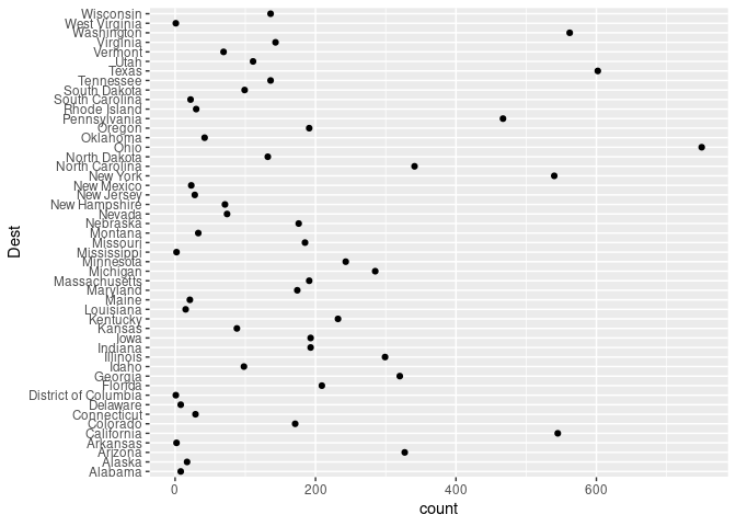

ggplot(arr_by_dest, aes(count, reorder(Dest, count))) + geom_point()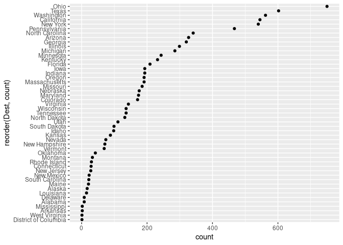

ggplot(slice_max(arr_by_dest, count, n = 5), aes(count, Dest)) + geom_point()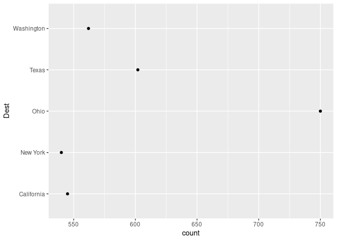


ggplot(arr_by_nat, aes(count, Nationality)) + geom_point()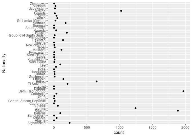

ggplot(arr_by_nat, aes(count, reorder(Nationality, count))) + geom_point()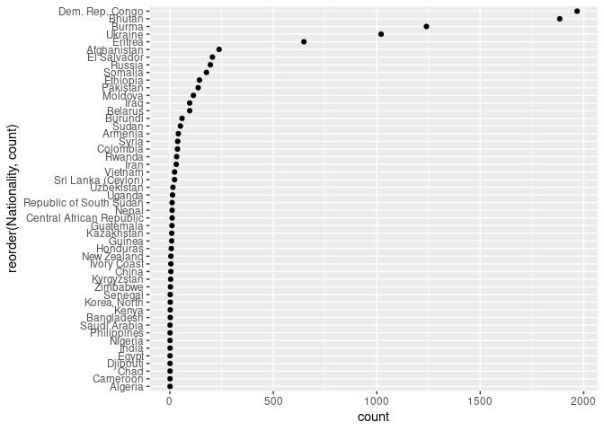

ggplot(slice_max(arr_by_nat, count, n = 5), aes(count, Nationality)) +
    geom_point()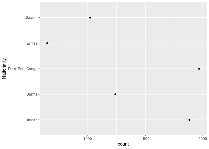

A useful visualization of flows is a Sankey diagram. These are also known as

alluvial diagrams;
river digrams;

and some would argue that allucial diagrams and river diagrams are different things.

Several R packages create these; including

alluvial
riverplot
googleVis.

This code creates a Sankey diagram using alluvial:

n_top <- 10
s_top <- 25

toprefs <- arrange(arr_by_nat, desc(count))$Nationality[1 : n_top]
topstates <- arrange(arr_by_dest, desc(count))$Dest[1 : s_top]

td3m <- mutate(td3,
               Nationality = ifelse(Nationality %in% toprefs,
                                    Nationality, "Other Nat."),
               Dest = ifelse(Dest %in% topstates, Dest, "Other Dest."))

std3m <- summarize(group_by(td3m, Dest, Nationality), count = sum(count))
## `summarise()` has grouped output by 'Dest'. You can override using the
## `.groups` argument.

pal <- c(rainbow(n_top), "grey")
pal <- c(RColorBrewer::brewer.pal(n_top, "Paired"), "grey")
src <- c(toprefs, "Other Nat.")

library(alluvial)
with(std3m, alluvial(Nationality, Dest, freq = count,
                     col = pal[match(Nationality, src)],
                     cex = 0.8, alpha = 0.7))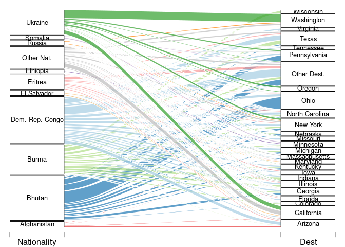

Another option is a chord diagram:

library(circlize)
chordDiagram(select(std3m, Nationality, Dest, count))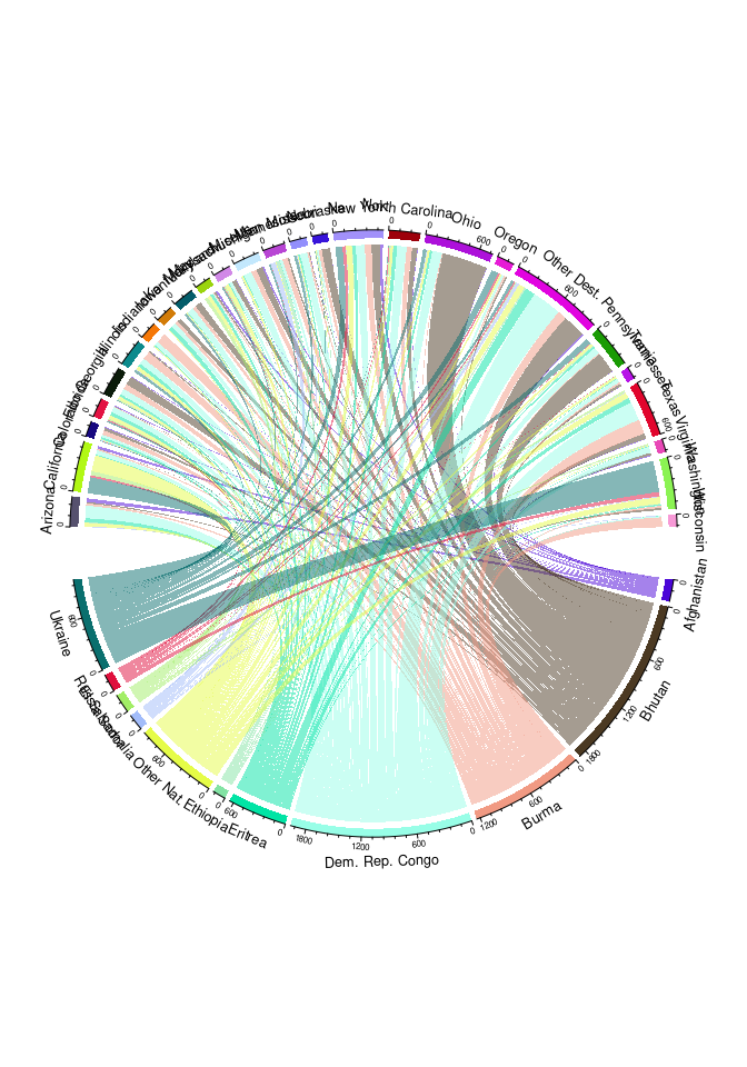

Gapminder Childhood Mortality Data

The gapminder package provides a subset of the data from the Gapminder web site. Additional data sets are available.

A data set on childhood mortality is available locally as a csv file or an Excel file.
The numbers represent number of deaths within the first five years per 1000 births.

Loading the data:

if (! file.exists("gapminder-under5mortality.xlsx"))
    download.file("http://homepage.stat.uiowa.edu/~luke/data/gapminder-under5mortality.xlsx", "gapminder-under5mortality.xlsx")
gcm <- read_excel("gapminder-under5mortality.xlsx")
names(gcm)[1]
## [1] "Under five mortality"
names(gcm)[1] <- "country"

A tidy version is useful for working with ggplot.

tgcm <- gather(gcm, year, u5mort, -1)
head(tgcm)
## # A tibble: 6 × 3
##   country               year   u5mort
##   <chr>                 <chr>   <dbl>
## 1 Abkhazia              1800.0    NA 
## 2 Afghanistan           1800.0   469.
## 3 Akrotiri and Dhekelia 1800.0    NA 
## 4 Albania               1800.0   375.
## 5 Algeria               1800.0   460.
## 6 American Samoa        1800.0    NA
tgcm <- mutate(tgcm, year = as.numeric(year))
head(tgcm)
## # A tibble: 6 × 3
##   country                year u5mort
##   <chr>                 <dbl>  <dbl>
## 1 Abkhazia               1800    NA 
## 2 Afghanistan            1800   469.
## 3 Akrotiri and Dhekelia  1800    NA 
## 4 Albania                1800   375.
## 5 Algeria                1800   460.
## 6 American Samoa         1800    NA

A multiple time series version may also be useful.

gcmts <- ts(t(gcm[-1]), start = 1800)
colnames(gcmts) <- gcm$country

Some explorations:

p <- ggplot(tgcm) + geom_line(aes(year, u5mort, group = country), alpha = 0.3)
p
## Warning: Removed 18644 rows containing missing values (`geom_line()`).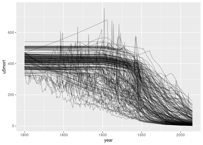

plotly::ggplotly(p)

xyplot(gcmts, superpose = TRUE, auto.key = FALSE)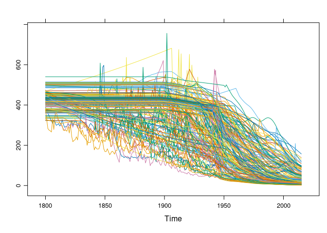

xyplot(gcmts, superpose = TRUE, auto.key = FALSE, col = "black")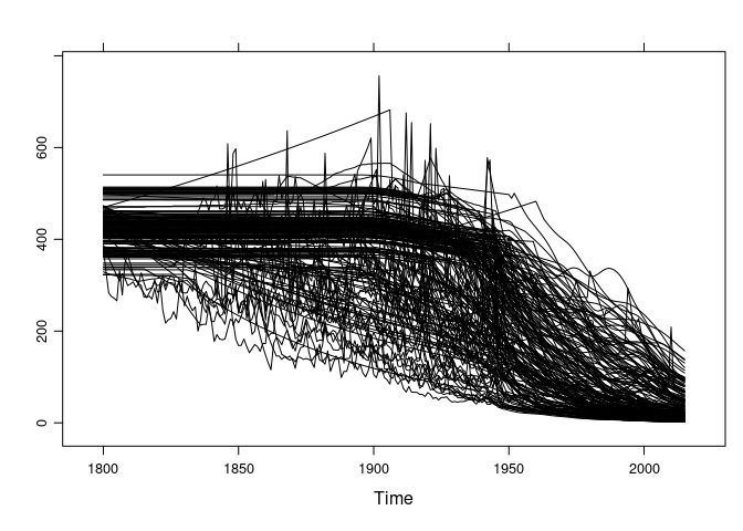

Examining the missing values:

anyNA(gcmts)
## [1] TRUE
sum(is.na(gcmts))
## [1] 18644
length(gcmts)
## [1] 59400

image(time(gcmts), seq_len(ncol(gcmts)), is.na(gcmts), ylab = "series")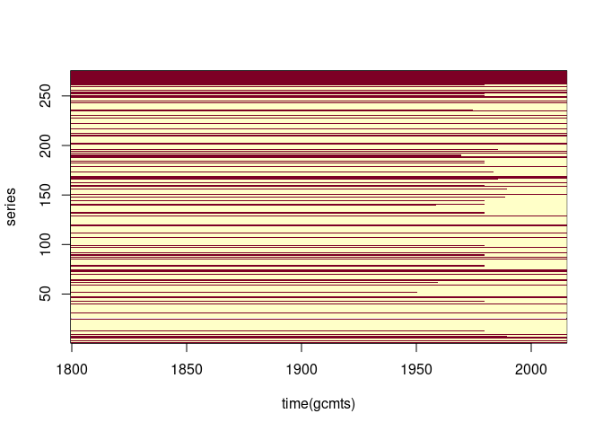

Re-ordering by the number of missing values may be useful:

naord <- order(apply(gcmts, 2, function(x) sum(is.na(x))))
image(time(gcmts), seq_len(ncol(gcmts)), is.na(gcmts)[, naord], ylab = "series")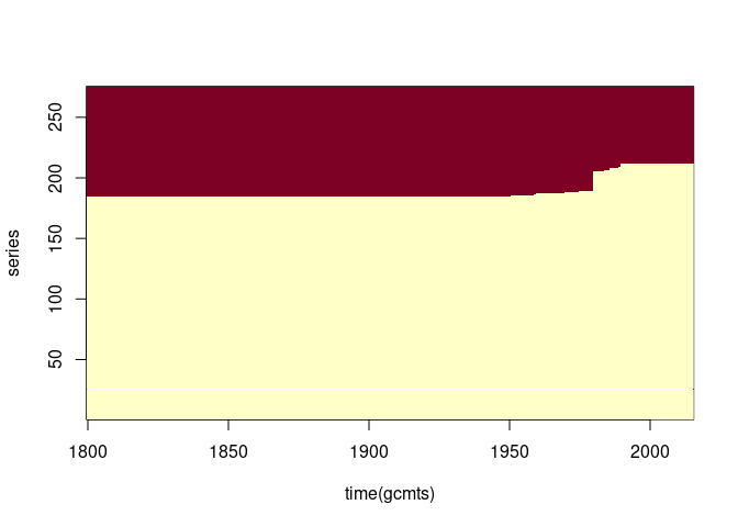

Some series look like the early values are estimates. Identifying and removing the ones that are constant between 1800 and 1850:

gcmtsNoNA <- gcmts[, ! apply(gcmts, 2, anyNA)]

i1850 <- which(time(gcmts) == 1850)
early_sd <- apply(gcmtsNoNA[1 : i1850, ], 2, sd)
filled_in <- names(which(early_sd == 0))

ggplot(filter(tgcm, ! country %in% filled_in)) +
    geom_line(aes(year, u5mort, group = country), alpha = 0.3, na.rm = TRUE)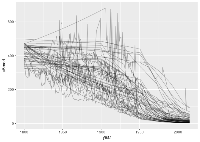

To show mortality rates by continent we can use the continent identification in the gapminder data set of the gapminder package.

There are a number of countries in the new data set not in gapminder

library(gapminder)
dim(gcm)
## [1] 275 217
length(unique(gapminder$country))
## [1] 142
head(setdiff(gcm$country, gapminder$country))
## [1] "Abkhazia"              "Akrotiri and Dhekelia" "American Samoa"       
## [4] "Andorra"               "Anguilla"              "Antigua and Barbuda"

There are several options for adding the continent information from gapminder to one of our data frames:

look-up using match
a left join or inner join using left_join
a left join or inner join using merge.

Using match, look up the index of the first row in gapminder for the country; then look up the corresponding continent:

cidx <- match(tgcm$country, gapminder$country)
head(cidx)
## [1] NA  1 NA 13 25 NA

cont <- gapminder$continent[cidx]
head(cont)
## [1] <NA>   Asia   <NA>   Europe Africa <NA>  
## Levels: Africa Americas Asia Europe Oceania

d1 <- mutate(tgcm, continent = cont)

Our left table will map country to continent, with one row per country:

country_continent <- unique(select(gapminder, country, continent))
head(country_continent)
## # A tibble: 6 × 2
##   country     continent
##   <fct>       <fct>    
## 1 Afghanistan Asia     
## 2 Albania     Europe   
## 3 Algeria     Africa   
## 4 Angola      Africa   
## 5 Argentina   Americas 
## 6 Australia   Oceania

The left join using left_join:

d2 <- left_join(tgcm, country_continent)
## Joining with `by = join_by(country)`

Joins in general may not produce the ordering you want; you need to check or make sure by reordering:

d1 <- arrange(d1, year, country)
d2 <- arrange(d2, year, country)
identical(unclass(d1), unclass(d2))
## [1] TRUE

The left join using merge:

d3 <- merge(tgcm, country_continent, all.x = TRUE)
d3 <- arrange(d3, year, country)
identical(d1, d3)
## [1] FALSE

Mapping continent to color:

ggplot(d3) +
    geom_line(aes(year, u5mort, group = country, color = continent),
              alpha = 0.7, na.rm = TRUE)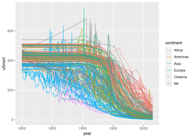

To compare child mortality to GDP per capita for the years covered by the gapminder data frame we need to merge the mortality data into gapminder.

Some country names in gapminder do not appear in the child mortality data:

setdiff(gapminder$country, tgcm$country)
## [1] "Korea, Dem. Rep." "Korea, Rep."      "Yemen, Rep."
grep("Korea", unique(tgcm$country), value = TRUE)
## [1] "North Korea"             "South Korea"            
## [3] "United Korea (former)\n"
grep("Yemen", unique(tgcm$country), value = TRUE)
## [1] "North Yemen (former)" "South Yemen (former)" "Yemen"

Change the names in tgcm`` to match the names ingapminder`:

ink <- which(tgcm$country == "North Korea")
isk <- which(tgcm$country == "South Korea")
iym <- which(tgcm$country == "Yemen")
tgcm$country[ink] <- "Korea, Dem. Rep."
tgcm$country[isk] <- "Korea, Rep."
tgcm$country[iym] <- "Yemen, Rep."

Now left join the mortality data with gapminder; the key is the combination of country and year:

Some plots:

gm <- left_join(gapminder, tgcm)
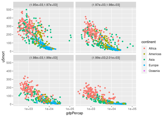
## Joining with `by = join_by(country, year)`

p <- ggplot(gm, aes(gdpPercap, u5mort, color = continent)) + geom_point()
p
## Warning: Removed 30 rows containing missing values (`geom_point()`).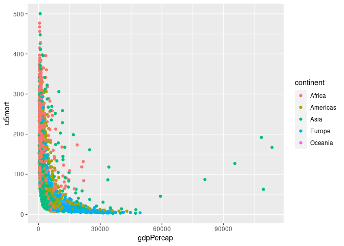

p + scale_x_log10()
## Warning: Removed 30 rows containing missing values (`geom_point()`).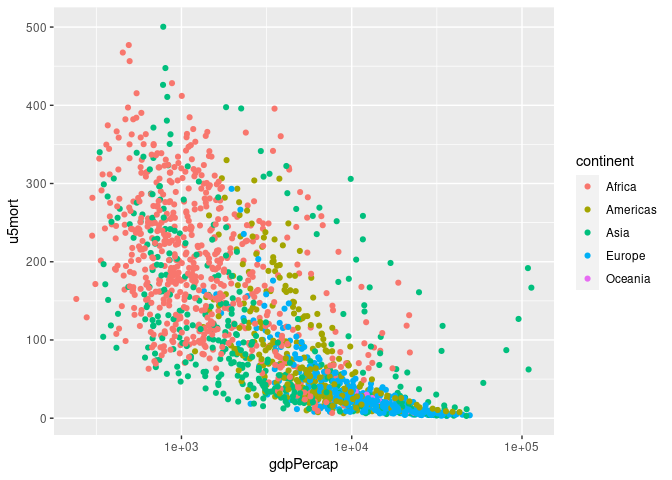

p + scale_x_log10() + facet_wrap(~ cut(year, 4))
## Warning: Removed 30 rows containing missing values (`geom_point()`).