
A Grammar of Data Manipulation
Background
The dplyr package provides a language, or grammar, for data manipulation.
The language contains a number of verbs that operate on tables in data frames.
The most commonly used verbs operate on a single data frame:
select(): pick variables by their namesfilter(): choose rows that satisfy some criteriamutate(): create transformed or derived variablesarrange(): reorder the rowssummarize(): collapse rows down to summaries
There are also a number of join verbs that merge several data frames into one.
The tidyr package provides additional verbs, such as pivot_longer() and pivot_wider() for reshaping data frames.
The single table verbs can also be used with group_by() and ungroup() to work a group at a time instead of applying to the entire data frame.
An experimental alternative to using group_by() and ungroup() is to use the .by argument with these verbs.
The design of dplyr is strongly motivated by SQL.
dplyrcan also be used to operate on tables stored in data bases.
The basic transformation verbs are described in the Data Transformation chapter of R for Data Science.
Utilities in tidyr are described in the Tidy Data chapter.
Some data sets for illustration:
EPA vehicle data used in HW4
library(readr)
if (! file.exists("vehicles.csv.zip"))
  download.file("http://www.stat.uiowa.edu/~luke/data/vehicles.csv.zip",
                "vehicles.csv.zip")
newmpg <- read_csv("vehicles.csv.zip", guess_max = 100000)
The
nycflights13package provides data on all flights originating from one of the three main New York City airports in 2013 and heading to airports within the US.library(nycflights13)The
anyflightspackage can be used to obtain data for other cities and periods.The
stormsdata frame, included indplyrwith data on hurricanes between 1975 and 2015.
Selecting Variables
Data sets often contain hundreds of even thousands of variables.
A useful first step is to select a group of interesting variables.
A reasonable selection of the EPA vehicle variables:
newmpg1 <- select(newmpg,
                  make, model, year,
                  cty = city08, hwy = highway08,
                  trans = trany, cyl = cylinders,
                  fuel = fuelType1, displ)
head(newmpg1, 2)
## # A tibble: 2 × 9
##   make       model               year   cty   hwy trans          cyl fuel  displ
##   <chr>      <chr>              <dbl> <dbl> <dbl> <chr>        <dbl> <chr> <dbl>
## 1 Alfa Romeo Spider Veloce 2000  1985    19    25 Manual 5-spd     4 Regu…   2
## 2 Ferrari    Testarossa          1985     9    14 Manual 5-spd    12 Regu…   4.9
Variables can be given new names in a select call; you can also rename them later with rename.
Some variations (the documentation for select() gives full details):
select(newmpg1, year : trans) |> head(2)
## # A tibble: 2 × 4
##    year   cty   hwy trans
##   <dbl> <dbl> <dbl> <chr>
## 1  1985    19    25 Manual 5-spd
## 2  1985     9    14 Manual 5-spd
select(newmpg1, -year, -trans) |> head(2)
## # A tibble: 2 × 7
## make model cty hwy cyl fuel displ
## <chr> <chr> <dbl> <dbl> <dbl> <chr> <dbl>
## 1 Alfa Romeo Spider Veloce 2000 19 25 4 Regular Gasoline 2
## 2 Ferrari Testarossa 9 14 12 Regular Gasoline 4.9select(newmpg1, - (year : trans)) |> head(2)
## # A tibble: 2 × 5
## make model cyl fuel displ
## <chr> <chr> <dbl> <chr> <dbl>
## 1 Alfa Romeo Spider Veloce 2000 4 Regular Gasoline 2
## 2 Ferrari Testarossa 12 Regular Gasoline 4.9Numerical column specifications can also be used:
select(newmpg1, 1, 3) |> head(2)
## # A tibble: 2 × 2
##   make        year
##   <chr>      <dbl>
## 1 Alfa Romeo  1985
## 2 Ferrari     1985
select(newmpg1, 1 : 3) |> head(2)
## # A tibble: 2 × 3
## make model year
## <chr> <chr> <dbl>
## 1 Alfa Romeo Spider Veloce 2000 1985
## 2 Ferrari Testarossa 1985select(newmpg1, - (1 : 3)) |> head(2)
## # A tibble: 2 × 6
## cty hwy trans cyl fuel displ
## <dbl> <dbl> <chr> <dbl> <chr> <dbl>
## 1 19 25 Manual 5-spd 4 Regular Gasoline 2
## 2 9 14 Manual 5-spd 12 Regular Gasoline 4.9Some helper functions can also be used in the column specifications.
The most useful ones are starts_with(), ends_with(), and contains().
select(newmpg, starts_with("fuel")) |> head(2)
## # A tibble: 2 × 5
##   fuelCost08 fuelCostA08 fuelType fuelType1        fuelType2
##        <dbl>       <dbl> <chr>    <chr>            <chr>
## 1       2200           0 Regular  Regular Gasoline <NA>
## 2       4150           0 Regular  Regular Gasoline <NA>
select(newmpg, contains("city")) |> head(2)
## # A tibble: 2 × 12
## city08 city08U cityA08 cityA08U cityCD cityE cityUF rangeCity rangeCityA UCity
## <dbl> <dbl> <dbl> <dbl> <dbl> <dbl> <dbl> <dbl> <dbl> <dbl>
## 1 19 0 0 0 0 0 0 0 0 23.3
## 2 9 0 0 0 0 0 0 0 0 11
## # ℹ 2 more variables: UCityA <dbl>, phevCity <dbl>By default these helpers ignore case.
These can also be preceded by a minus modifier to omit columns:
select(newmpg1, -contains("m")) |> head(2)
## # A tibble: 2 × 7
##    year   cty   hwy trans          cyl fuel             displ
##   <dbl> <dbl> <dbl> <chr>        <dbl> <chr>            <dbl>
## 1  1985    19    25 Manual 5-spd     4 Regular Gasoline   2
## 2  1985     9    14 Manual 5-spd    12 Regular Gasoline   4.9
contains requires a literal string; matches() is analogous but its argument is interpreted as a regular expression pattern to be matched.
select(newmpg, matches("^[Ff]uel")) |> head(2)
## # A tibble: 2 × 5
##   fuelCost08 fuelCostA08 fuelType fuelType1        fuelType2
##        <dbl>       <dbl> <chr>    <chr>            <chr>
## 1       2200           0 Regular  Regular Gasoline <NA>
## 2       4150           0 Regular  Regular Gasoline <NA>
Sometimes it is useful to move a few columns to the front; the everything() helper can be used for that.
The original NYC flights table:
head(flights, 2)
## # A tibble: 2 × 19
##    year month   day dep_time sched_dep_time dep_delay arr_time sched_arr_time
##   <int> <int> <int>    <int>          <int>     <dbl>    <int>          <int>
## 1  2013     1     1      517            515         2      830            819
## 2  2013     1     1      533            529         4      850            830
## # ℹ 11 more variables: arr_delay <dbl>, carrier <chr>, flight <int>,
## #   tailnum <chr>, origin <chr>, dest <chr>, air_time <dbl>, distance <dbl>,
## #   hour <dbl>, minute <dbl>, time_hour <dttm>
Moving air_time to the front:
select(flights, air_time, everything()) |> head(2)
## # A tibble: 2 × 19
##   air_time  year month   day dep_time sched_dep_time dep_delay arr_time
##      <dbl> <int> <int> <int>    <int>          <int>     <dbl>    <int>
## 1      227  2013     1     1      517            515         2      830
## 2      227  2013     1     1      533            529         4      850
## # ℹ 11 more variables: sched_arr_time <int>, arr_delay <dbl>, carrier <chr>,
## #   flight <int>, tailnum <chr>, origin <chr>, dest <chr>, distance <dbl>,
## #   hour <dbl>, minute <dbl>, time_hour <dttm>
The where() helper function allows columns to be selected based on a predicate applied to the full column:
select(newmpg1, where(anyNA)) |> head(2)
## # A tibble: 2 × 3
##   trans          cyl displ
##   <chr>        <dbl> <dbl>
## 1 Manual 5-spd     4   2
## 2 Manual 5-spd    12   4.9
select(flights, where(anyNA)) |> head(2)
## # A tibble: 2 × 6
## dep_time dep_delay arr_time arr_delay tailnum air_time
## <int> <dbl> <int> <dbl> <chr> <dbl>
## 1 517 2 830 11 N14228 227
## 2 533 4 850 20 N24211 227If there are missing values in your data it is usually a good idea to review them to make sure you understand what they mean.
Columns can also be selected using list operations:
vars <- c("make", "model", "year", "city08", "trany", "cylinders",
          "fuelType1", "displ")
newmpg[vars] |> head(2)
## # A tibble: 2 × 8
##   make       model               year city08 trany     cylinders fuelType1 displ
##   <chr>      <chr>              <dbl>  <dbl> <chr>         <dbl> <chr>     <dbl>
## 1 Alfa Romeo Spider Veloce 2000  1985     19 Manual 5…         4 Regular …   2
## 2 Ferrari    Testarossa          1985      9 Manual 5…        12 Regular …   4.9
Filtering Rows
The filter() function picks out the subset of rows that satisfy one or more conditions.
All cars with city MPG at or above 140 and model year 2024:
filter(newmpg1, cty >= 140, year == 2024)
## # A tibble: 3 × 9
##   make    model                         year   cty   hwy trans   cyl fuel  displ
##   <chr>   <chr>                        <dbl> <dbl> <dbl> <chr> <dbl> <chr> <dbl>
## 1 Hyundai Ioniq 6 Long range RWD (18 …  2024   153   127 Auto…    NA Elec…    NA
## 2 Hyundai Ioniq 6 Standard Range RWD    2024   151   120 Auto…    NA Elec…    NA
## 3 Lucid   Air Pure RWD with 19 inch w…  2024   140   134 Auto…    NA Elec…    NA
All flights from New York to Des Moines on January 1, 2013:
filter(flights, day == 1, month == 1, dest == "DSM") |>
    select(year : dep_time, origin)
## # A tibble: 1 × 5
##    year month   day dep_time origin
##   <int> <int> <int>    <int> <chr>
## 1  2013     1     1     2119 EWR
Comparisons
The basic comparison operators are
==,!=<,<=>,>=
Be sure to use ==, not a single = character.
Be careful about floating point equality tests:
x <- 1 - 0.9
x == 0.1
## [1] FALSE
near(x, 0.1)
## [1] TRUE
Equality comparisons can be used on character vectors and factors.
Order comparisons can be used on character vectors, but may produce surprising results, or results that vary with different locale settings.
%in% can be used to match against one of several options:
filter(flights, day %in% 1 : 2, month == 1, dest == "DSM") |>
    select(year : dep_time, origin)
## # A tibble: 2 × 5
##    year month   day dep_time origin
##   <int> <int> <int>    <int> <chr>
## 1  2013     1     1     2119 EWR
## 2  2013     1     2     1921 EWR
Logical Operations
The basic logical operations on vectors are
&– and|– or!– notxor– exclusive or
Truth tables:
x <- c(TRUE, TRUE,  FALSE, FALSE)
y <- c(TRUE, FALSE, TRUE,  FALSE)
! x
## [1] FALSE FALSE  TRUE  TRUE
x & y
## [1]  TRUE FALSE FALSE FALSE
x | y
## [1]  TRUE  TRUE  TRUE FALSE
xor(x, y)
## [1] FALSE  TRUE  TRUE FALSE
Make sure not to confuse the vectorized logical operators & and | with the scalar flow control operators && and ||.
The previous flights example can also be written as
filter(flights, day == 1 | day == 2, month == 1, dest == "DSM") |>
    select(year : dep_time, origin)
## # A tibble: 2 × 5
##    year month   day dep_time origin
##   <int> <int> <int>    <int> <chr>
## 1  2013     1     1     2119 EWR
## 2  2013     1     2     1921 EWR
It can also be written as
filter(flights, (day == 1 | day == 2) & month == 1 & dest == "DSM") |>
    select(year : dep_time, origin)
## # A tibble: 2 × 5
##    year month   day dep_time origin
##   <int> <int> <int>    <int> <chr>
## 1  2013     1     1     2119 EWR
## 2  2013     1     2     1921 EWR
Missing Values
filter() only keeps values corresponding to TRUE predicate values; FALSE and NA values are dropped.
Arithmetic and comparison operators will always produce NA values if one operand is NA.
1 + NA
## [1] NA
NA < 1
## [1] NA
NA == NA
## [1] NA
In a few cases a non-NA result can be determined:
TRUE | NA
## [1] TRUE
NA & FALSE
## [1] FALSE
NA ^ 0
## [1] 1
is.na() can be used to also select rows with NA values.
Non-electric vehicles with zero or NA for displ:
filter(newmpg1, displ == 0 | is.na(displ), fuel != "Electricity")
## # A tibble: 2 × 9
##   make   model     year   cty   hwy trans          cyl fuel             displ
##   <chr>  <chr>    <dbl> <dbl> <dbl> <chr>        <dbl> <chr>            <dbl>
## 1 Subaru RX Turbo  1985    22    28 Manual 5-spd    NA Regular Gasoline    NA
## 2 Subaru RX Turbo  1985    21    27 Manual 5-spd    NA Regular Gasoline    NA
Flights with NA for both dep_time and arr_time:
filter(flights, is.na(dep_time) & is.na(arr_time)) |>
    select(year : arr_time)
## # A tibble: 8,255 × 7
##     year month   day dep_time sched_dep_time dep_delay arr_time
##    <int> <int> <int>    <int>          <int>     <dbl>    <int>
##  1  2013     1     1       NA           1630        NA       NA
##  2  2013     1     1       NA           1935        NA       NA
##  3  2013     1     1       NA           1500        NA       NA
##  4  2013     1     1       NA            600        NA       NA
##  5  2013     1     2       NA           1540        NA       NA
##  6  2013     1     2       NA           1620        NA       NA
##  7  2013     1     2       NA           1355        NA       NA
##  8  2013     1     2       NA           1420        NA       NA
##  9  2013     1     2       NA           1321        NA       NA
## 10  2013     1     2       NA           1545        NA       NA
## # ℹ 8,245 more rows
An alternative approach that does not use filter would be
idx <- with(flights, is.na(dep_time) & is.na(arr_time))
flights[idx, ] |>
    select(year : arr_time)
## # A tibble: 8,255 × 7
##     year month   day dep_time sched_dep_time dep_delay arr_time
##    <int> <int> <int>    <int>          <int>     <dbl>    <int>
##  1  2013     1     1       NA           1630        NA       NA
##  2  2013     1     1       NA           1935        NA       NA
##  3  2013     1     1       NA           1500        NA       NA
##  4  2013     1     1       NA            600        NA       NA
##  5  2013     1     2       NA           1540        NA       NA
##  6  2013     1     2       NA           1620        NA       NA
##  7  2013     1     2       NA           1355        NA       NA
##  8  2013     1     2       NA           1420        NA       NA
##  9  2013     1     2       NA           1321        NA       NA
## 10  2013     1     2       NA           1545        NA       NA
## # ℹ 8,245 more rows
Exploring the EPA Data
Sorting out fuel types:
select(newmpg, contains("fuelType")) |> unique()
## # A tibble: 14 × 3
##    fuelType                    fuelType1         fuelType2
##    <chr>                       <chr>             <chr>
##  1 Regular                     Regular Gasoline  <NA>
##  2 Premium                     Premium Gasoline  <NA>
##  3 Diesel                      Diesel            <NA>
##  4 CNG                         Natural Gas       <NA>
##  5 Gasoline or natural gas     Regular Gasoline  Natural Gas
##  6 Gasoline or E85             Regular Gasoline  E85
##  7 Electricity                 Electricity       <NA>
##  8 Gasoline or propane         Regular Gasoline  Propane
##  9 Premium or E85              Premium Gasoline  E85
## 10 Midgrade                    Midgrade Gasoline <NA>
## 11 Premium Gas or Electricity  Premium Gasoline  Electricity
## 12 Regular Gas and Electricity Regular Gasoline  Electricity
## 13 Premium and Electricity     Premium Gasoline  Electricity
## 14 Regular Gas or Electricity  Regular Gasoline  Electricity
Variables with missing values:
select(newmpg, where(anyNA)) |> head(2)
## # A tibble: 2 × 17
##   cylinders displ drive      eng_dscr trany guzzler trans_dscr tCharger sCharger
##       <dbl> <dbl> <chr>      <chr>    <chr> <chr>   <chr>      <lgl>    <chr>
## 1         4   2   Rear-Whee… (FFS)    Manu… <NA>    <NA>       NA       <NA>
## 2        12   4.9 Rear-Whee… (GUZZLE… Manu… T       <NA>       NA       <NA>
## # ℹ 8 more variables: atvType <chr>, fuelType2 <chr>, rangeA <chr>,
## #   evMotor <chr>, mfrCode <chr>, c240Dscr <chr>, c240bDscr <chr>,
## #   startStop <chr>
Among the reduced data set:
select(newmpg1, where(anyNA)) |> names()
## [1] "trans" "cyl"   "displ"
Unique missing value patterns:
incomplete_cases <- function(data) data[! complete.cases(data), ]

select(newmpg1, trans, cyl, displ, fuel) |>
    incomplete_cases() |>
    unique()
## # A tibble: 9 × 4
##   trans                              cyl displ fuel
##   <chr>                            <dbl> <dbl> <chr>
## 1 <NA>                                NA  NA   Electricity
## 2 <NA>                                 8   5.8 Regular Gasoline
## 3 <NA>                                 6   4.1 Regular Gasoline
## 4 Manual 5-spd                        NA  NA   Regular Gasoline
## 5 Manual 5-spd                        NA   1.3 Regular Gasoline
## 6 Automatic (A1)                      NA  NA   Electricity
## 7 Automatic (variable gear ratios)    NA  NA   Electricity
## 8 Automatic (A1)                      NA   0   Electricity
## 9 Automatic (A2)                      NA  NA   Electricity
An alternative to defining incomplete_cases():
select(newmpg1, trans, cyl, displ, fuel) |>
    filter(if_any(everything(), is.na)) |>
    unique()
## # A tibble: 9 × 4
##   trans                              cyl displ fuel
##   <chr>                            <dbl> <dbl> <chr>
## 1 <NA>                                NA  NA   Electricity
## 2 <NA>                                 8   5.8 Regular Gasoline
## 3 <NA>                                 6   4.1 Regular Gasoline
## 4 Manual 5-spd                        NA  NA   Regular Gasoline
## 5 Manual 5-spd                        NA   1.3 Regular Gasoline
## 6 Automatic (A1)                      NA  NA   Electricity
## 7 Automatic (variable gear ratios)    NA  NA   Electricity
## 8 Automatic (A1)                      NA   0   Electricity
## 9 Automatic (A2)                      NA  NA   Electricity
Looking at the counts:
select(newmpg1, trans, cyl, displ, fuel) |>
    incomplete_cases() |>
    count(trans, cyl, displ, fuel)
## # A tibble: 9 × 5
##   trans                              cyl displ fuel                 n
##   <chr>                            <dbl> <dbl> <chr>            <int>
## 1 Automatic (A1)                      NA   0   Electricity          1
## 2 Automatic (A1)                      NA  NA   Electricity        567
## 3 Automatic (A2)                      NA  NA   Electricity         63
## 4 Automatic (variable gear ratios)    NA  NA   Electricity          9
## 5 Manual 5-spd                        NA   1.3 Regular Gasoline     1
## 6 Manual 5-spd                        NA  NA   Regular Gasoline     2
## 7 <NA>                                 6   4.1 Regular Gasoline     1
## 8 <NA>                                 8   5.8 Regular Gasoline     1
## 9 <NA>                                NA  NA   Electricity          9
count(trans, cyl, displ, fuel) is essentially an abbreviation of
group_by(trans, cyl, displ, fuel) |>
    summarize(n = n()) |>
    ungroup()
Another approach that avoids specifying the variables with missing values:
incomplete_cases(newmpg1) |>
    count(across(where(anyNA)), fuel)
## # A tibble: 9 × 5
##   trans                              cyl displ fuel                 n
##   <chr>                            <dbl> <dbl> <chr>            <int>
## 1 Automatic (A1)                      NA   0   Electricity          1
## 2 Automatic (A1)                      NA  NA   Electricity        567
## 3 Automatic (A2)                      NA  NA   Electricity         63
## 4 Automatic (variable gear ratios)    NA  NA   Electricity          9
## 5 Manual 5-spd                        NA   1.3 Regular Gasoline     1
## 6 Manual 5-spd                        NA  NA   Regular Gasoline     2
## 7 <NA>                                 6   4.1 Regular Gasoline     1
## 8 <NA>                                 8   5.8 Regular Gasoline     1
## 9 <NA>                                NA  NA   Electricity          9
Cylinders for electric vehicles:
filter(newmpg1, fuel == "Electricity") |>
    count(is.na(cyl))
## # A tibble: 1 × 2
##   `is.na(cyl)`     n
##   <lgl>        <int>
## 1 TRUE           649
Displacement for electric vehicles:
filter(newmpg1, fuel == "Electricity") |>
    count(is.na(displ))
## # A tibble: 2 × 2
##   `is.na(displ)`     n
##   <lgl>          <int>
## 1 FALSE              1
## 2 TRUE             648
Electric vehicles with non-missing displacement:
filter(newmpg1, fuel == "Electricity", ! is.na(displ))
## # A tibble: 1 × 9
##   make       model   year   cty   hwy trans            cyl fuel        displ
##   <chr>      <chr>  <dbl> <dbl> <dbl> <chr>          <dbl> <chr>       <dbl>
## 1 Mitsubishi i-MiEV  2016   126    99 Automatic (A1)    NA Electricity     0
Some things to think about for electric vehicles:
Should electric vehicles be dropped from analyses or visualizations involving cylinders or displacement?
Should
cylordisplbe recoded, perhaps as zero?Why are miles per gallon not missing, or infinite, for electric vehicles? The documentation for the data has some pointers.
Other considerations:
Should some transmission levels be combined?
Should some fuel type levels be combined?
Adding New Variables
mutate() can be used to define new variables or modify existing ones.
New variables are added at the end.
Later variables can be defined in terms of earlier ones.
mutate() does not modify the original data frame; it creates a new one with the specified modifications.
fl <- select(flights, year, month, day, air_time, ends_with("delay"))
mutate(fl,
       gain = dep_delay - arr_delay,
       air_hours = air_time / 60,
       gain_per_hour = gain / air_hours) |>
    head(2)
## # A tibble: 2 × 9
##    year month   day air_time dep_delay arr_delay  gain air_hours gain_per_hour
##   <int> <int> <int>    <dbl>     <dbl>     <dbl> <dbl>     <dbl>         <dbl>
## 1  2013     1     1      227         2        11    -9      3.78         -2.38
## 2  2013     1     1      227         4        20   -16      3.78         -4.23
transmute() keeps only the new variables.
transmute(flights,
          gain = dep_delay - arr_delay,
          air_hours = air_time / 60,
          gain_per_hour = gain / air_hours) |>
    head(2)
## # A tibble: 2 × 3
##    gain air_hours gain_per_hour
##   <dbl>     <dbl>         <dbl>
## 1    -9      3.78         -2.38
## 2   -16      3.78         -4.23
Useful operators include:
Basic arithmetic operators, logarithms, etc.
Modular arithmetic operators
%/%and%%Logical operators and comparison operators.
Offset operators
lead()andlag().cumulative aggregates such as
cumsum(),cummean().Ranking operators, such as
min_rank(),percent_rank().Predicates like
is.na.
A reasonable guess is that flights with NA values for both dep_time and arr_time were cancelled:
fl <- mutate(flights,
             cancelled = is.na(dep_time) & is.na(arr_time))
For the geyser data set from the MASS package we used lag to obtain the duration of the previous eruption,
data(geyser, package = "MASS")
geyser2 <- mutate(geyser,
                  prev_duration = lag(duration))
head(geyser2, 4)
##   waiting duration prev_duration
## 1      80 4.016667            NA
## 2      71 2.150000      4.016667
## 3      57 4.000000      2.150000
## 4      80 4.000000      4.000000
thm <- theme_minimal() +
theme(text = element_text(size = 16))
ggplot(geyser2) +
geom_point(aes(x = prev_duration,
y = waiting)) +
thm## Warning: Removed 1 row containing missing values or values outside the scale range
## (`geom_point()`).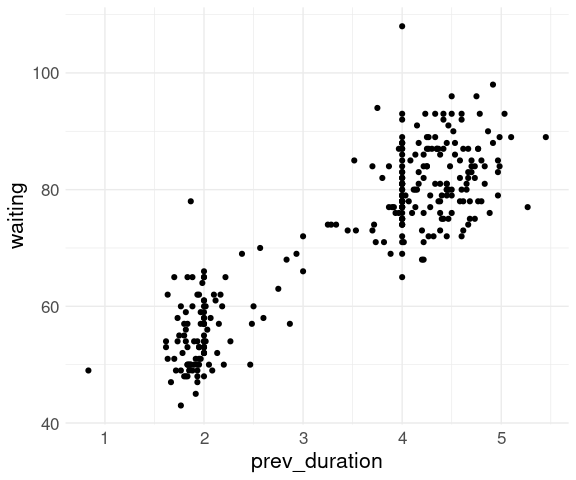
The top five vehicles in cty gas mileage (there may be more than five if there is a tie for fifth place):
mutate(newmpg1, cty_rank = min_rank(desc(cty))) |>
    filter(cty_rank <= 5)
## # A tibble: 8 × 10
##   make    model                year   cty   hwy trans   cyl fuel  displ cty_rank
##   <chr>   <chr>               <dbl> <dbl> <dbl> <chr> <dbl> <chr> <dbl>    <int>
## 1 Hyundai Ioniq Electric       2017   150   122 Auto…    NA Elec…    NA        5
## 2 Hyundai Ioniq Electric       2018   150   122 Auto…    NA Elec…    NA        5
## 3 Hyundai Ioniq Electric       2019   150   122 Auto…    NA Elec…    NA        5
## 4 Tesla   Model 3 Standard R…  2021   150   133 Auto…    NA Elec…    NA        5
## 5 Hyundai Ioniq 6 Long range…  2023   153   127 Auto…    NA Elec…    NA        1
## 6 Hyundai Ioniq 6 Standard R…  2023   151   120 Auto…    NA Elec…    NA        3
## 7 Hyundai Ioniq 6 Long range…  2024   153   127 Auto…    NA Elec…    NA        1
## 8 Hyundai Ioniq 6 Standard R…  2024   151   120 Auto…    NA Elec…    NA        3
An alternative to explicitly computing ranks and filtering is the slice_max() utility function:
slice_max(newmpg1, cty, n = 5)
## # A tibble: 8 × 9
##   make    model                         year   cty   hwy trans   cyl fuel  displ
##   <chr>   <chr>                        <dbl> <dbl> <dbl> <chr> <dbl> <chr> <dbl>
## 1 Hyundai Ioniq 6 Long range RWD (18 …  2023   153   127 Auto…    NA Elec…    NA
## 2 Hyundai Ioniq 6 Long range RWD (18 …  2024   153   127 Auto…    NA Elec…    NA
## 3 Hyundai Ioniq 6 Standard Range RWD    2023   151   120 Auto…    NA Elec…    NA
## 4 Hyundai Ioniq 6 Standard Range RWD    2024   151   120 Auto…    NA Elec…    NA
## 5 Hyundai Ioniq Electric                2017   150   122 Auto…    NA Elec…    NA
## 6 Hyundai Ioniq Electric                2018   150   122 Auto…    NA Elec…    NA
## 7 Hyundai Ioniq Electric                2019   150   122 Auto…    NA Elec…    NA
## 8 Tesla   Model 3 Standard Range Plus…  2021   150   133 Auto…    NA Elec…    NA
The percent_rank function produces a ‘percentile rank’ (but between 0 and 1).
The top 5% of countries in life expectancy in 2007 from the gapminder data set:
library(gapminder)
gm <- filter(gapminder, year == 2007)
gm_top <- filter(gm, percent_rank(desc(lifeExp)) <= 0.05)
gm_top
## # A tibble: 8 × 6
##   country          continent  year lifeExp       pop gdpPercap
##   <fct>            <fct>     <int>   <dbl>     <int>     <dbl>
## 1 Australia        Oceania    2007    81.2  20434176    34435.
## 2 Hong Kong, China Asia       2007    82.2   6980412    39725.
## 3 Iceland          Europe     2007    81.8    301931    36181.
## 4 Israel           Asia       2007    80.7   6426679    25523.
## 5 Japan            Asia       2007    82.6 127467972    31656.
## 6 Spain            Europe     2007    80.9  40448191    28821.
## 7 Sweden           Europe     2007    80.9   9031088    33860.
## 8 Switzerland      Europe     2007    81.7   7554661    37506.
And the bottom 5%:
filter(gm, percent_rank(lifeExp) <= 0.05)
## # A tibble: 8 × 6
##   country      continent  year lifeExp      pop gdpPercap
##   <fct>        <fct>     <int>   <dbl>    <int>     <dbl>
## 1 Afghanistan  Asia       2007    43.8 31889923      975.
## 2 Angola       Africa     2007    42.7 12420476     4797.
## 3 Lesotho      Africa     2007    42.6  2012649     1569.
## 4 Mozambique   Africa     2007    42.1 19951656      824.
## 5 Sierra Leone Africa     2007    42.6  6144562      863.
## 6 Swaziland    Africa     2007    39.6  1133066     4513.
## 7 Zambia       Africa     2007    42.4 11746035     1271.
## 8 Zimbabwe     Africa     2007    43.5 12311143      470.
Within these results the original row order is retained.
The arrange function can be used to change this.
Arranging Rows
arrange() reorders the rows according to one or more variables.
By default the order is smallest to largest; using desc() reverses this.
Additional variables will be used to break ties.
Arranging the top 5% of countries in life expectancy in 2007 by life expectancy:
arrange(gm_top, desc(lifeExp))
## # A tibble: 8 × 6
##   country          continent  year lifeExp       pop gdpPercap
##   <fct>            <fct>     <int>   <dbl>     <int>     <dbl>
## 1 Japan            Asia       2007    82.6 127467972    31656.
## 2 Hong Kong, China Asia       2007    82.2   6980412    39725.
## 3 Iceland          Europe     2007    81.8    301931    36181.
## 4 Switzerland      Europe     2007    81.7   7554661    37506.
## 5 Australia        Oceania    2007    81.2  20434176    34435.
## 6 Spain            Europe     2007    80.9  40448191    28821.
## 7 Sweden           Europe     2007    80.9   9031088    33860.
## 8 Israel           Asia       2007    80.7   6426679    25523.
To order by continent name and order by life expectancy within continent:
arrange(gm_top, continent, desc(lifeExp))
## # A tibble: 8 × 6
##   country          continent  year lifeExp       pop gdpPercap
##   <fct>            <fct>     <int>   <dbl>     <int>     <dbl>
## 1 Japan            Asia       2007    82.6 127467972    31656.
## 2 Hong Kong, China Asia       2007    82.2   6980412    39725.
## 3 Israel           Asia       2007    80.7   6426679    25523.
## 4 Iceland          Europe     2007    81.8    301931    36181.
## 5 Switzerland      Europe     2007    81.7   7554661    37506.
## 6 Spain            Europe     2007    80.9  40448191    28821.
## 7 Sweden           Europe     2007    80.9   9031088    33860.
## 8 Australia        Oceania    2007    81.2  20434176    34435.
Missing values are sorted to the end:
df <- data.frame(x = c(5, 2, NA, 3))
arrange(df, x)
##    x
## 1  2
## 2  3
## 3  5
## 4 NA
arrange(df, desc(x))
##    x
## 1  5
## 2  3
## 3  2
## 4 NA
Using is.na you can arrange to put them at the beginning:
arrange(df, desc(is.na(x)), x)
##    x
## 1 NA
## 2  2
## 3  3
## 4  5
Summarizing and Grouping
summarize() collapses a table down to one row of summaries.
The average and maximal departure and arrival delays for flights, along with the total number of flights:
summarize(flights,
          ave_dep_delay = mean(dep_delay, na.rm = TRUE),
          ave_arr_delay = mean(arr_delay, na.rm = TRUE),
          max_dep_delay = max(dep_delay, na.rm = TRUE),
          max_arr_delay = max(arr_delay, na.rm = TRUE),
          n = n())
## # A tibble: 1 × 5
##   ave_dep_delay ave_arr_delay max_dep_delay max_arr_delay      n
##           <dbl>         <dbl>         <dbl>         <dbl>  <int>
## 1          12.6          6.90          1301          1272 336776
Grouped Summaries
summarize() is most commonly used with grouped data to provide group level summaries.
Grouping delay summaries by destination:
fl_dest <-
    group_by(flights, dest) |>
    summarize(ave_dep_delay = mean(dep_delay, na.rm = TRUE),
              ave_arr_delay = mean(arr_delay, na.rm = TRUE),
              max_dep_delay = max(dep_delay, na.rm = TRUE),
              max_arr_delay = max(arr_delay, na.rm = TRUE),
              n = n()) |>
    ungroup()
head(fl_dest, 5)
## # A tibble: 5 × 6
##   dest  ave_dep_delay ave_arr_delay max_dep_delay max_arr_delay     n
##   <chr>         <dbl>         <dbl>         <dbl>         <dbl> <int>
## 1 ABQ           13.7           4.38           142           153   254
## 2 ACK            6.46          4.85           219           221   265
## 3 ALB           23.6          14.4            323           328   439
## 4 ANC           12.9          -2.5             75            39     8
## 5 ATL           12.5          11.3            898           895 17215
Calling ungroup is not always necessary but sometimes it is, so it is a good habit to get into.
An alternative to using group_by() and ungroup() is to use the .by argument to summarize():
flights |>
    summarize(ave_dep_delay = mean(dep_delay, na.rm = TRUE),
              ave_arr_delay = mean(arr_delay, na.rm = TRUE),
              max_dep_delay = max(dep_delay, na.rm = TRUE),
              max_arr_delay = max(arr_delay, na.rm = TRUE),
              n = n(),
              .by = dest) |>
    arrange(dest) |>      ## to match group_by() result
    head()
## # A tibble: 6 × 6
##   dest  ave_dep_delay ave_arr_delay max_dep_delay max_arr_delay     n
##   <chr>         <dbl>         <dbl>         <dbl>         <dbl> <int>
## 1 ABQ           13.7           4.38           142           153   254
## 2 ACK            6.46          4.85           219           221   265
## 3 ALB           23.6          14.4            323           328   439
## 4 ANC           12.9          -2.5             75            39     8
## 5 ATL           12.5          11.3            898           895 17215
## 6 AUS           13.0           6.02           351           349  2439
This is currently marked as Experimental in the documentation.
The group level summaries can be further transformed, for example to identify the top 10 destinations for average delays:
mutate(fl_dest, rank = min_rank(desc(ave_dep_delay))) |>
    filter(rank <= 10)
## # A tibble: 10 × 7
##    dest  ave_dep_delay ave_arr_delay max_dep_delay max_arr_delay     n  rank
##    <chr>         <dbl>         <dbl>         <dbl>         <dbl> <int> <int>
##  1 ALB            23.6          14.4           323           328   439     9
##  2 BHM            29.7          16.9           325           291   297     4
##  3 CAE            35.6          41.8           222           224   116     1
##  4 DSM            26.2          19.0           341           322   569     7
##  5 JAC            26.5          28.1           198           175    25     6
##  6 MSN            23.6          20.2           340           364   572    10
##  7 OKC            30.6          30.6           280           262   346     3
##  8 RIC            23.6          20.1           483           463  2454     8
##  9 TUL            34.9          33.7           251           262   315     2
## 10 TYS            28.5          24.1           291           281   631     5
Missing Values
Most summaries will be NA if any of the data values being summarized are NA.
Typically, summary functions can be called with na.rm = TRUE to produce the summary for all non-missing values.
summarize(flights,
          ave_dep_delay = mean(dep_delay, na.rm = TRUE),
          ave_arr_delay = mean(arr_delay, na.rm = TRUE),
          max_dep_delay = max(dep_delay, na.rm = TRUE),
          max_arr_delay = max(arr_delay, na.rm = TRUE),
          n = n())
## # A tibble: 1 × 5
##   ave_dep_delay ave_arr_delay max_dep_delay max_arr_delay      n
##           <dbl>         <dbl>         <dbl>         <dbl>  <int>
## 1          12.6          6.90          1301          1272 336776
You can also use filter() to remove rows with NA values in the variables to be summarized:
filter(flights, ! is.na(dep_delay), ! is.na(arr_delay)) |>
    summarize(ave_dep_delay = mean(dep_delay),
              ave_arr_delay = mean(arr_delay),
              max_dep_delay = max(dep_delay),
              max_arr_delay = max(arr_delay),
              n = n())
## # A tibble: 1 × 5
##   ave_dep_delay ave_arr_delay max_dep_delay max_arr_delay      n
##           <dbl>         <dbl>         <dbl>         <dbl>  <int>
## 1          12.6          6.90          1301          1272 327346
The two approaches do produce different counts.
Counts
The helper function n() provides a count of the number of rows in the table being summarized.
Including counts with grouped summaries is usually a good idea.
Summaries based on small counts are likely to be much less reliable than ones based on larger counts.
This is reflected in higher variability among averages for destinations with fewer flights:
ggplot(fl_dest) +
    geom_point(aes(x = n,
                   y = ave_arr_delay),
               na.rm = TRUE) +
    thm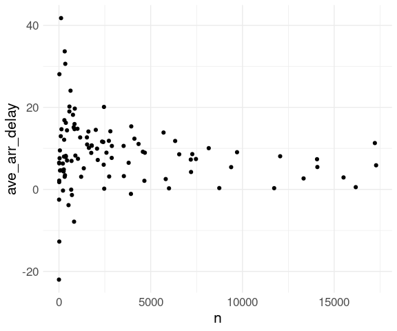
A plotly version allows the individual destinations to be identified easily:
library(plotly)
p <- ggplot(fl_dest) +
    geom_point(aes(x = n,
                   y = ave_arr_delay,
                   text = dest),
               na.rm = FALSE) +
    thm
ggplotly(p, tooltip = "text")
It would be more user-friendly to show the airport name than the three letter FAA code.
Useful Summaries
Some useful summary functions:
Location:
mean(),median()Spread:
sd(),IQR(),mad()Rank:
min(),quantile(),max()Position:
first(),nth(),last()Counts:
n().
Airline Arrival Delays
Different Delay Measures
Sometimes it is useful to look at subsets or truncated versions of a variable.
Airlines like to arrange schedules so they are often early.
ggplot(flights, aes(x = arr_delay,
                    y = after_stat(density))) +
    geom_histogram(binwidth = 1,
                   na.rm = TRUE,
                   fill = "deepskyblue3") +
    xlim(c(-100, 250)) +
    thm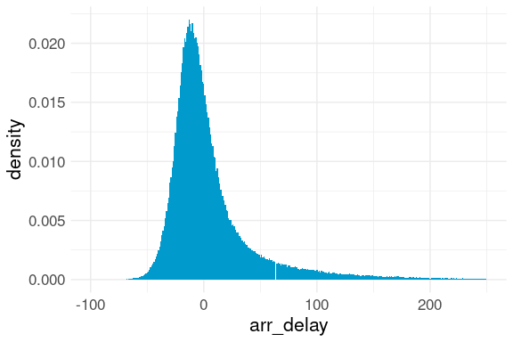
This reduces the average arrival delay but may not help travelers much.
Two options:
Consider only the positive delays for the average.
Treat negative delays as zero (zero-truncation).
The mean of the positive delays can be computed using subsetting:
mean(arr_delay[arr_delay > 0])The mean of the zero-truncated delays can be computed using the pmax function:
mean(pmax(arr_delay, 0))The summaries are
fl_arr <- filter(flights, ! is.na(arr_delay))
fl_avs <-
    group_by(fl_arr, dest) |>
    summarize(ave = mean(arr_delay),
              ave_pos = mean(arr_delay[arr_delay > 0]),
              ave_pos_zero = mean(pmax(arr_delay, 0)),
              n = n()) |>
    ungroup()
head(fl_avs)
## # A tibble: 6 × 5
##   dest    ave ave_pos ave_pos_zero     n
##   <chr> <dbl>   <dbl>        <dbl> <int>
## 1 ABQ    4.38    41.9        17.7    254
## 2 ACK    4.85    28.6        11.3    264
## 3 ALB   14.4     52.1        22.9    418
## 4 ANC   -2.5     12.4         7.75     8
## 5 ATL   11.3     37.8        17.8  16837
## 6 AUS    6.02    40.6        16.6   2411
One approach to visualizing the results with color coding the three different summaries:
View the
fl_avstable as a wide format withavs,ave_pos, andave_pos_zeroas three different measurement types.Use
pivot_longer()to convert to a long format with a variablewhichto hold the summary type and a variabledelayto hold the summary value:
library(tidyr)
fl <- pivot_longer(fl_avs, 2 : 4,
                   names_to = "which",
                   values_to = "delay")
arrange(fl, dest)
## # A tibble: 312 × 4
##    dest      n which        delay
##    <chr> <int> <chr>        <dbl>
##  1 ABQ     254 ave           4.38
##  2 ABQ     254 ave_pos      41.9
##  3 ABQ     254 ave_pos_zero 17.7
##  4 ACK     264 ave           4.85
##  5 ACK     264 ave_pos      28.6
##  6 ACK     264 ave_pos_zero 11.3
##  7 ALB     418 ave          14.4
##  8 ALB     418 ave_pos      52.1
##  9 ALB     418 ave_pos_zero 22.9
## 10 ANC       8 ave          -2.5
## # ℹ 302 more rows
A plot is then easy to create:
ggplot(fl, aes(x = n,
               y = delay,
               color = which)) +
    geom_point() +
    thm
## Warning: Removed 1 row containing missing values or values outside the scale range
## (`geom_point()`).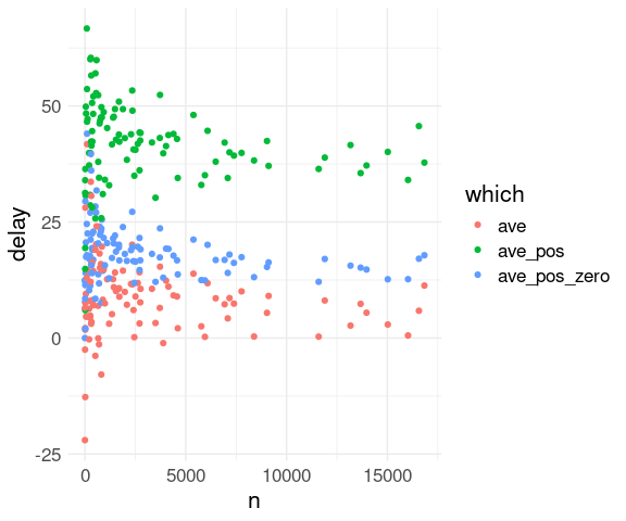
An alternative:
Use one layer per summary type.
Specify the summary type for each layer as a
coloraesthetic value.
ggplot(fl_avs, aes(x = n)) +
    geom_point(aes(y = ave,
                   color = "ave")) +
    geom_point(aes(y = ave_pos,
                   color = "ave_pos")) +
    geom_point(aes(y = ave_pos_zero,
                   color = "ave_pos_zero")) +
    thm
## Warning: Removed 1 row containing missing values or values outside the scale range
## (`geom_point()`).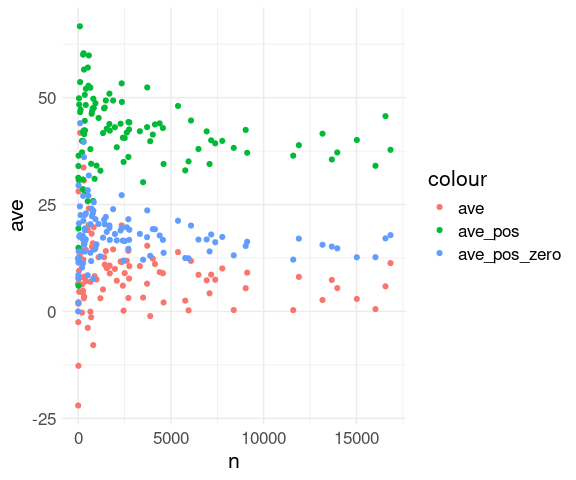
The one missing value case:
incomplete_cases(fl_avs)
## # A tibble: 1 × 5
##   dest    ave ave_pos ave_pos_zero     n
##   <chr> <dbl>   <dbl>        <dbl> <int>
## 1 LEX     -22     NaN            0     1
Delay Proportions
Proportions satisfying a condition can be computed as a mean of the logical expression for the condition:
The proportion of all flights that were delayed:
mean(fl_arr$arr_delay > 0)
## [1] 0.4063101
Grouped by destination:
fl_props <-
    group_by(fl_arr, dest) |>
    summarize(
        pd0 = mean(arr_delay > 0),   ## proportion delayed
        pd10 = mean(arr_delay > 10), ## more than 10 minutes
        pd20 = mean(arr_delay > 20), ## more than 20 minutes
        n = n()) |>
    ungroup()
fl_props
## # A tibble: 104 × 5
##    dest    pd0  pd10  pd20     n
##    <chr> <dbl> <dbl> <dbl> <int>
##  1 ABQ   0.421 0.339 0.268   254
##  2 ACK   0.394 0.246 0.167   264
##  3 ALB   0.440 0.333 0.273   418
##  4 ANC   0.625 0.125 0.125     8
##  5 ATL   0.472 0.309 0.211 16837
##  6 AUS   0.408 0.284 0.216  2411
##  7 AVL   0.456 0.257 0.207   261
##  8 BDL   0.350 0.262 0.223   412
##  9 BGR   0.383 0.299 0.246   358
## 10 BHM   0.450 0.361 0.305   269
## # ℹ 94 more rows
These can be visualized similarly:
pivot_longer(fl_props, 2 : 4,
             names_to = "which",
             values_to = "prop") |>
    ggplot(aes(x = n,
               y = prop,
               color = which)) +
    geom_point() +
    thm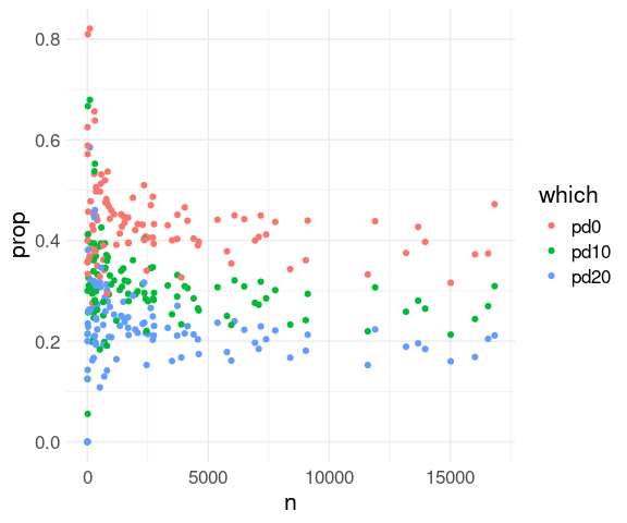
Grouped Mutate and Filter
mutate(), filter(), arrange(), slice_max(), and slice_min() can be used on a group level.
Standardizing Within Groups
mutate within groups can be used for standardizing within a group.
For example, to compute the proportion of a continent’s population living in each country for each year:
gm <- group_by(gapminder, continent, year) |>
    mutate(ppop = pop / sum(pop)) |>
    ungroup()
Using the .by argument to mutate():
gm2 <- mutate(gapminder, ppop = pop / sum(pop), .by = c(continent, year))
identical(gm, gm2)
## [1] TRUE
For Oceania (in this data set) and years 1952 and 2007:
gm_oc <- filter(gm, continent == "Oceania", year %in% c(1952, 2007)) |>
    arrange(year)
gm_oc
## # A tibble: 4 × 7
##   country     continent  year lifeExp      pop gdpPercap  ppop
##   <fct>       <fct>     <int>   <dbl>    <int>     <dbl> <dbl>
## 1 Australia   Oceania    1952    69.1  8691212    10040. 0.813
## 2 New Zealand Oceania    1952    69.4  1994794    10557. 0.187
## 3 Australia   Oceania    2007    81.2 20434176    34435. 0.832
## 4 New Zealand Oceania    2007    80.2  4115771    25185. 0.168
A quick check that within year and continent the proportions add up to one:
group_by(gm_oc, continent, year) |> summarize(sum_ppop = sum(ppop))
## # A tibble: 2 × 3
## # Groups:   continent [1]
##   continent  year sum_ppop
##   <fct>     <int>    <dbl>
## 1 Oceania    1952        1
## 2 Oceania    2007        1
Focus on the 2 countries in each continent with the highest proportions of the continent’s population:
gmt2 <- group_by(gm, continent, year) |>
    slice_max(ppop, n = 2) |>
    ungroup() |>
    filter(continent != "Oceania") ## drop as there are only two
ggplot(gmt2, aes(x = year, y = ppop,
                 group = country, color = country)) +
    geom_line() + geom_point() +
    facet_wrap(~ continent, scales = "free_y") +
    thm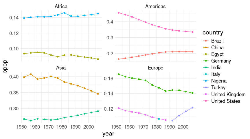
Another approach:
Create separate plots for each continent.
Adjust the themes a little.
Use
facet_wrap()to get the facet label.Arrange the plots, e.g. using
patchworkoperators.
A useful feature is that the %+% operator can be used to change the base data frame for a plot:
pAf <- ggplot(filter(gmt2, continent == "Africa"),
              aes(x = year, y = ppop, col = country)) +
    geom_line() + geom_point() +
    facet_wrap(~ continent) +
    thm +
    theme(legend.position = "top",
          legend.title = element_blank())
thm_nx <- theme(axis.title.x = element_blank())
thm_ny <- theme(axis.title.y = element_blank())
pAm <- pAf %+% filter(gmt2, continent == "Americas")
pAs <- pAf %+% filter(gmt2, continent == "Asia")
pEu <- pAf %+% filter(gmt2, continent == "Europe") +
    guides(color = guide_legend(nrow = 2))
library(patchwork)
((pAf + thm_nx) | (pAm + thm_nx + thm_ny)) /
    (pAs | (pEu + thm_ny))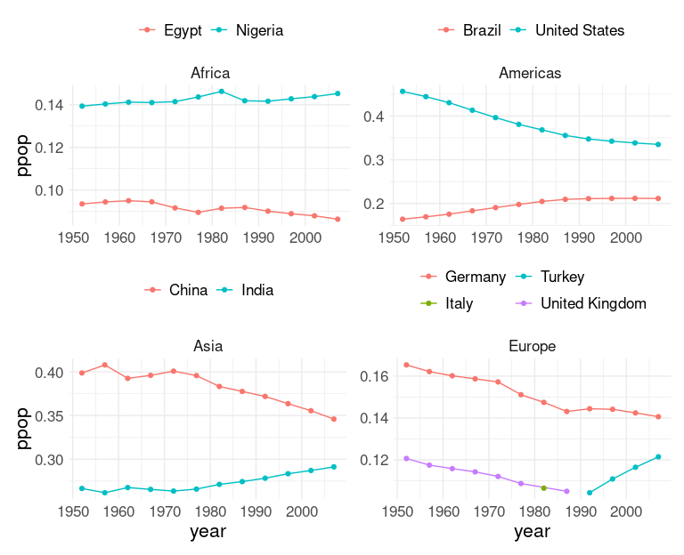
Changes Over Time
Changes over time within a country can also be examined with a grouped mutate and the lag operator.
For variables collected over time the lag function can be used to compute the previous value of a variable:
gm_us <- filter(gapminder,
                country == "United States") |>
    transmute(year,
              lifeExp,
              prev_lifeExp = lag(lifeExp))
gm_us
## # A tibble: 12 × 3
##     year lifeExp prev_lifeExp
##    <int>   <dbl>        <dbl>
##  1  1952    68.4         NA
##  2  1957    69.5         68.4
##  3  1962    70.2         69.5
##  4  1967    70.8         70.2
##  5  1972    71.3         70.8
##  6  1977    73.4         71.3
##  7  1982    74.6         73.4
##  8  1987    75.0         74.6
##  9  1992    76.1         75.0
## 10  1997    76.8         76.1
## 11  2002    77.3         76.8
## 12  2007    78.2         77.3
This can then be used to compute the change from one period to the next:
mutate(gm_us,
       le_change = lifeExp - prev_lifeExp)
## # A tibble: 12 × 4
##     year lifeExp prev_lifeExp le_change
##    <int>   <dbl>        <dbl>     <dbl>
##  1  1952    68.4         NA      NA
##  2  1957    69.5         68.4     1.05
##  3  1962    70.2         69.5     0.720
##  4  1967    70.8         70.2     0.550
##  5  1972    71.3         70.8     0.580
##  6  1977    73.4         71.3     2.04
##  7  1982    74.6         73.4     1.27
##  8  1987    75.0         74.6     0.370
##  9  1992    76.1         75.0     1.07
## 10  1997    76.8         76.1     0.720
## 11  2002    77.3         76.8     0.5
## 12  2007    78.2         77.3     0.932
Use this idea to compute changes in lifeExp and gdpPercap for all countries in a grouped mutate:
gm <- group_by(gapminder, country) |>
    mutate(
        le_change = lifeExp - lag(lifeExp),
        gdp_change = gdpPercap - lag(gdpPercap),
        gdp_pct_change =
            100 * gdp_change / lag(gdpPercap)) |>
    ungroup()
slice_max() can then be applied to data grouped by country to extract the rows with the highest gdp_pct_change for each country:
group_by(gm, country) |>
    slice_max(gdp_pct_change, n = 1) |>
    ungroup() |>
    select(1 : 3, contains("gdp"))
## # A tibble: 142 × 6
##    country     continent  year gdpPercap gdp_change gdp_pct_change
##    <fct>       <fct>     <int>     <dbl>      <dbl>          <dbl>
##  1 Afghanistan Asia       2007      975.       248.           34.1
##  2 Albania     Europe     2002     4604.      1411.           44.2
##  3 Algeria     Africa     1972     4183.       936.           28.8
##  4 Angola      Africa     2007     4797.      2024.           73.0
##  5 Argentina   Americas   2007    12779.      3982.           45.3
##  6 Australia   Oceania    1967    14526.      2309.           18.9
##  7 Austria     Europe     1957     8843.      2706.           44.1
##  8 Bahrain     Asia       2007    29796.      6392.           27.3
##  9 Bangladesh  Asia       2007     1391.       255.           22.4
## 10 Belgium     Europe     1972    16672.      3523.           26.8
## # ℹ 132 more rows
Grouping by continent allows the worst drop in life expectancy for each continent to be found:
group_by(gm, continent) |>
    slice_min(le_change, n = 1) |>
    ungroup() |>
    select(-contains("gdp"))
## # A tibble: 5 × 6
##   country     continent  year lifeExp      pop le_change
##   <fct>       <fct>     <int>   <dbl>    <int>     <dbl>
## 1 Rwanda      Africa     1992    23.6  7290203   -20.4
## 2 El Salvador Americas   1977    56.7  4282586    -1.51
## 3 Cambodia    Asia       1977    31.2  6978607    -9.10
## 4 Montenegro  Europe     2002    74.0   720230    -1.46
## 5 Australia   Oceania    1967    71.1 11872264     0.170
Without grouping, the row with best percent GDP change overall can be computed:
slice_max(gm, gdp_pct_change, n = 1) |>
    select(country, continent, year, gdp_pct_change)
## # A tibble: 1 × 4
##   country continent  year gdp_pct_change
##   <fct>   <fct>     <int>          <dbl>
## 1 Libya   Africa     1967           178.
The computation of the best GDP growth years by country can be combined into a single pipe:
group_by(gapminder, country) |>
    mutate(gdp_change = gdpPercap - lag(gdpPercap),
           gdp_pct_change = 100 * gdp_change / lag(gdpPercap)) |>
    ungroup() |>
    group_by(country) |>
    slice_max(gdp_pct_change, n = 1) |>
    ungroup() |>
    select(1 : 3, contains("gdp"))
Since the groupings of the two steps are the same and grouped mutate preserves the group structure, the middle ungroup/group_by can be dropped:
group_by(gapminder, country) |>
    mutate(gdp_change = gdpPercap - lag(gdpPercap),
           gdp_pct_change = 100 * gdp_change / lag(gdpPercap)) |>
    slice_max(gdp_pct_change, n = 1) |>
    ungroup() |>
    select(1 : 3, contains("gdp"))
You need to be very careful making an optimization like this!
Joins
This interactive plot uses the tooltip to show the airport code for the destination:
library(plotly)
p <- ggplot(fl_dest) +
    geom_point(aes(x = n,
                   y = ave_arr_delay,
                   text = dest)) +
    thm
## Warning in geom_point(aes(x = n, y = ave_arr_delay, text = dest)): Ignoring
## unknown aesthetics: text
ggplotly(p, tooltip = "text")
A nicer approach would be to show the airport name.
The airports table provides this information:
head(airports, 2)
## # A tibble: 2 × 8
##   faa   name                            lat   lon   alt    tz dst   tzone
##   <chr> <chr>                         <dbl> <dbl> <dbl> <dbl> <chr> <chr>
## 1 04G   Lansdowne Airport              41.1 -80.6  1044    -5 A     America/New…
## 2 06A   Moton Field Municipal Airport  32.5 -85.7   264    -6 A     America/Chi…
We need to get this information into the fl_dest data frame.
As another example, we might want to explore whether aircraft age is related to delays.
The planes table provides the year of manufacture:
head(planes, 2)
## # A tibble: 2 × 9
##   tailnum  year type               manufacturer model engines seats speed engine
##   <chr>   <int> <chr>              <chr>        <chr>   <int> <int> <int> <chr>
## 1 N10156   2004 Fixed wing multi … EMBRAER      EMB-…       2    55    NA Turbo…
## 2 N102UW   1998 Fixed wing multi … AIRBUS INDU… A320…       2   182    NA Turbo…
Again, we need to merge this information with the data in the flights table.
One way to do this is with a join operation.
Joins are a common operation in data bases.
Murell’s Data Technologies book describes data bases in Section 5.6 and data base queries using SQL in Chapter 7.
R for Data Science describes relational data in Chapter 13.
dplyr distinguishes between two kinds of joins:
mutating joins;
filtering joins.
These animated explanations may be helpful.
Mutating Joins
Mutating joins combine variables and rows from two tables by matching rows on keys.
A primary key is a variable, or combination of variables, in a table that uniquely identify the rows of the table.
A foreign key is a variable, or combination of variables, that uniquely identify a row in some table (usually, but not necessarily, a different table).
The simplest join operation is an inner join: Only rows for which the key appears in both tables are retained.
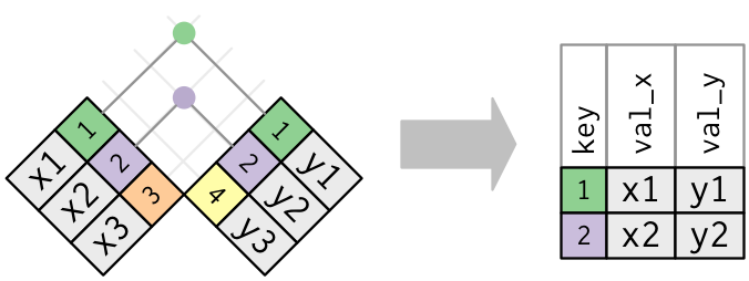
Outer joins retain some other rows with NA values for new variables:
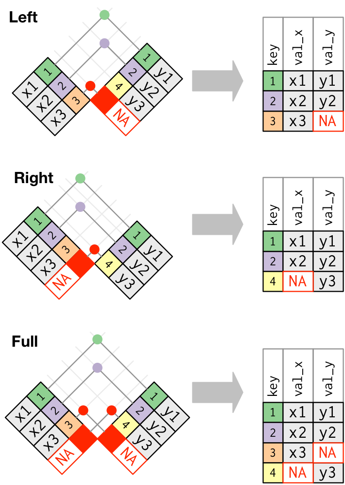
Inner and left joins are the most common.
The key of one of the tables should usually be a primary key that uniquely identifies the table’s rows.
For a left join, the right table key should usually use a primary key.
It is usually a good idea to make sure a primary key candidate really does uniquely identify rows.
For the planes table the tailnum variable is a primary key;
count(planes, tailnum) |> filter(n > 1)
## # A tibble: 0 × 2
## # ℹ 2 variables: tailnum <chr>, n <int>
For the flights data a primary key needs to use multiple variables.
A reasonable guess is to use the date, carrier and flight number, but this isn’t quite enough:
count(flights, year, month, day, flight, carrier) |>
    filter(n > 1) |>
    head(2)
## # A tibble: 2 × 6
##    year month   day flight carrier     n
##   <int> <int> <int>  <int> <chr>   <int>
## 1  2013     6     8   2269 WN          2
## 2  2013     6    15   2269 WN          2
Adding the origin airport code does produce a primary key:
count(flights, year, month, day, flight, carrier, origin) |>
    filter(n > 1)
## # A tibble: 0 × 7
## # ℹ 7 variables: year <int>, month <int>, day <int>, flight <int>,
## #   carrier <chr>, origin <chr>, n <int>
To relate delays to aircraft age we can start with summaries by tailnum and year (year would be needed if we had data for more than 2013):
fl <- filter(flights, ! is.na(dep_time), ! is.na(arr_time)) |>
    group_by(year, tailnum) |>
    summarize(ave_dep_delay = mean(dep_delay, na.rm = TRUE),
              ave_arr_delay = mean(arr_delay, na.rm = TRUE),
              n = n()) |>
    ungroup()
head(fl)
## # A tibble: 6 × 5
## year tailnum ave_dep_delay ave_arr_delay n
## <int> <chr> <dbl> <dbl> <int>
## 1 2013 D942DN 31.5 31.5 4
## 2 2013 N0EGMQ 8.49 9.98 354
## 3 2013 N10156 17.8 12.7 146
## 4 2013 N102UW 8 2.94 48
## 5 2013 N103US -3.20 -6.93 46
## 6 2013 N104UW 10.1 1.80 46A reduced planes table with year renamed to avoid a conflict:
pl <- select(planes, tailnum, plane_year = year)pl
## # A tibble: 3,322 × 2
## tailnum plane_year
## <chr> <int>
## 1 N10156 2004
## 2 N102UW 1998
## 3 N103US 1999
## 4 N104UW 1999
## 5 N10575 2002
## 6 N105UW 1999
## 7 N107US 1999
## 8 N108UW 1999
## 9 N109UW 1999
## 10 N110UW 1999
## # ℹ 3,312 more rowsNow
use a left join with
tailnumas the key to bring theplane_yearvalue into the summary tableand then compute the plane age:
fl_age <- left_join(fl, pl, "tailnum") |>
    mutate(plane_age = year - plane_year)
fl_age
## # A tibble: 4,037 × 7
##     year tailnum ave_dep_delay ave_arr_delay     n plane_year plane_age
##    <int> <chr>           <dbl>         <dbl> <int>      <int>     <int>
##  1  2013 D942DN         31.5          31.5       4         NA        NA
##  2  2013 N0EGMQ          8.49          9.98    354         NA        NA
##  3  2013 N10156         17.8          12.7     146       2004         9
##  4  2013 N102UW          8             2.94     48       1998        15
##  5  2013 N103US         -3.20         -6.93     46       1999        14
##  6  2013 N104UW         10.1           1.80     46       1999        14
##  7  2013 N10575         22.3          20.7     271       2002        11
##  8  2013 N105UW          2.58         -0.267    45       1999        14
##  9  2013 N107US         -0.463        -5.73     41       1999        14
## 10  2013 N108UW          4.22         -1.25     60       1999        14
## # ℹ 4,027 more rows
An initial plot:
ggplot(fl_age,
       aes(x = plane_age,
           y = ave_dep_delay)) +
    geom_point() +
    thm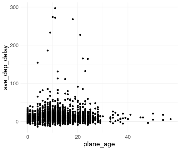
Jittering and adjusting the point size may help:
ggplot(fl_age,
       aes(x = plane_age,
           y = ave_dep_delay)) +
    geom_point(position = "jitter",
               size = 0.1) +
    thm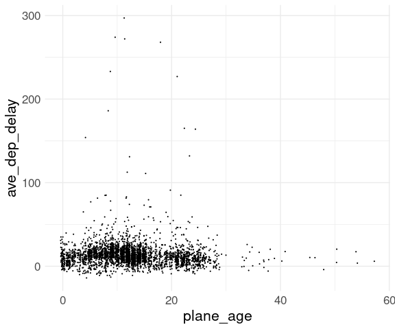
Adding a smooth and adjusting the ranges may also help:
ggplot(fl_age,
       aes(x = plane_age,
           y = ave_dep_delay)) +
    geom_point(position = "jitter",
               size = 0.1) +
    geom_smooth() +
    xlim(0, 30) +
    ylim(c(-20, 80)) +
    thm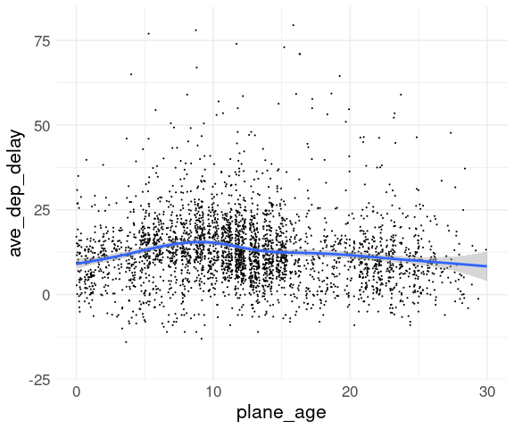
Another option is to compute means or medians within years:
flm <- group_by(fl_age, plane_age) |>
    summarize(ave_dep_delay =
                  mean(ave_dep_delay,
                       na.rm = TRUE)) |>
    ungroup()
ggplot(flm,
       aes(x = plane_age,
           y = ave_dep_delay)) +
    geom_point(na.rm = TRUE) +
    thm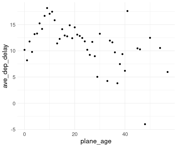
Both the smooth and the means show a modest increase over the first 10 years.
A left join can also be used to add the airport name from the airport table to the fl_dest table.
The primary key in the airport table is the three-letter airport code in the faa variable:
head(airports, 2)
## # A tibble: 2 × 8
##   faa   name                            lat   lon   alt    tz dst   tzone
##   <chr> <chr>                         <dbl> <dbl> <dbl> <dbl> <chr> <chr>
## 1 04G   Lansdowne Airport              41.1 -80.6  1044    -5 A     America/New…
## 2 06A   Moton Field Municipal Airport  32.5 -85.7   264    -6 A     America/Chi…
The foreign key in the fl_dest table to match is the dest variable:
head(fl_dest, 2)
## # A tibble: 2 × 6
##   dest  ave_dep_delay ave_arr_delay max_dep_delay max_arr_delay     n
##   <chr>         <dbl>         <dbl>         <dbl>         <dbl> <int>
## 1 ABQ           13.7           4.38           142           153   254
## 2 ACK            6.46          4.85           219           221   265
The left_join function allows this link to be made by specifying the key as c("dest" = "faa"):
fl_dest <- left_join(fl_dest,
                     select(airports, faa, dest_name = name),
                     c("dest" = "faa"))
select(fl_dest, dest_name, everything())
## # A tibble: 105 × 7
##    dest_name dest  ave_dep_delay ave_arr_delay max_dep_delay max_arr_delay     n
##    <chr>     <chr>         <dbl>         <dbl>         <dbl>         <dbl> <int>
##  1 Albuquer… ABQ           13.7           4.38           142           153   254
##  2 Nantucke… ACK            6.46          4.85           219           221   265
##  3 Albany I… ALB           23.6          14.4            323           328   439
##  4 Ted Stev… ANC           12.9          -2.5             75            39     8
##  5 Hartsfie… ATL           12.5          11.3            898           895 17215
##  6 Austin B… AUS           13.0           6.02           351           349  2439
##  7 Ashevill… AVL            8.19          8.00           222           228   275
##  8 Bradley … BDL           17.7           7.05           252           266   443
##  9 Bangor I… BGR           19.5           8.03           248           238   375
## 10 Birmingh… BHM           29.7          16.9            325           291   297
## # ℹ 95 more rows
Now a tooltip can provide a more accessible label:
p <- ggplot(fl_dest) +
    geom_point(aes(x = n,
                   y = ave_arr_delay,
                   text = paste(dest,
                                dest_name,
                                sep = ": "))) +
    thm
ggplotly(p, tooltip = "text")
Filtering Joins
Filtering joins only affect rows; they do not add variables.
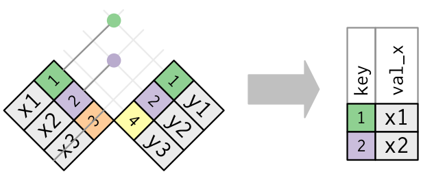
semi_join(x, y)returns all rows inxwith a match iny:
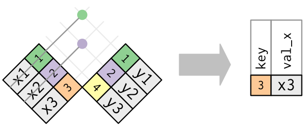
anti_join(x, y)returns all rows inxwithout a match iny:
semi_join is useful for matching filtered results back to a table.
The plot of delay against age showed some surprisingly old aircraft:
top_age <- slice_max(fl_age, plane_age, n = 2)
top_age
## # A tibble: 3 × 7
##    year tailnum ave_dep_delay ave_arr_delay     n plane_year plane_age
##   <int> <chr>           <dbl>         <dbl> <int>      <int>     <int>
## 1  2013 N381AA           5.95          3.5     22       1956        57
## 2  2013 N201AA          17.4          14.1     51       1959        54
## 3  2013 N567AA           3.72         -4.30    61       1959        54
We can identify these aircraft with a semi-join:
semi_join(planes, top_age, "tailnum")
## # A tibble: 3 × 9
##   tailnum  year type               manufacturer model engines seats speed engine
##   <chr>   <int> <chr>              <chr>        <chr>   <int> <int> <int> <chr>
## 1 N201AA   1959 Fixed wing single… CESSNA       150         1     2    90 Recip…
## 2 N381AA   1956 Fixed wing multi … DOUGLAS      DC-7…       4   102   232 Recip…
## 3 N567AA   1959 Fixed wing single… DEHAVILLAND  OTTE…       1    16    95 Recip…
The corresponding flights can also be picked out with a semi-join:
top_age_flights <- semi_join(flights, top_age, "tailnum")
head(top_age_flights, 2)
## # A tibble: 2 × 19
##    year month   day dep_time sched_dep_time dep_delay arr_time sched_arr_time
##   <int> <int> <int>    <int>          <int>     <dbl>    <int>          <int>
## 1  2013     1     3      909            700       129     1103            850
## 2  2013     1     3       NA            920        NA       NA           1245
## # ℹ 11 more variables: arr_delay <dbl>, carrier <chr>, flight <int>,
## #   tailnum <chr>, origin <chr>, dest <chr>, air_time <dbl>, distance <dbl>,
## #   hour <dbl>, minute <dbl>, time_hour <dttm>
Looking at the carriers or destinations might help:
select(top_age_flights, carrier, dest, everything()) |> head(4)
## # A tibble: 4 × 19
##   carrier dest   year month   day dep_time sched_dep_time dep_delay arr_time
##   <chr>   <chr> <int> <int> <int>    <int>          <int>     <dbl>    <int>
## 1 AA      ORD    2013     1     3      909            700       129     1103
## 2 AA      DFW    2013     1     3       NA            920        NA       NA
## 3 AA      DFW    2013     1     9     1423           1430        -7     1727
## 4 AA      DFW    2013     1    10     1238           1240        -2     1525
## # ℹ 10 more variables: sched_arr_time <int>, arr_delay <dbl>, flight <int>,
## #   tailnum <chr>, origin <chr>, air_time <dbl>, distance <dbl>, hour <dbl>,
## #   minute <dbl>, time_hour <dttm>
The carrier summary:
count(top_age_flights, carrier)
## # A tibble: 1 × 2
##   carrier     n
##   <chr>   <int>
## 1 AA        139
A check of the documentation for planes shows that American and one other airline report fleet numbers rather than tail numbers.
Anti-joins are useful for detecting join problems.
For example, many flights have tail numbers that do not match entries in planes:
fl <- anti_join(flights, planes, "tailnum")
nrow(fl)
## [1] 52606
count(fl, tailnum)
## # A tibble: 722 × 2
## tailnum n
## <chr> <int>
## 1 D942DN 4
## 2 N0EGMQ 371
## 3 N14628 1
## 4 N149AT 22
## 5 N16632 11
## 6 N17627 2
## 7 N1EAMQ 210
## 8 N200AA 34
## 9 N24633 8
## 10 N261AV 6
## # ℹ 712 more rowsJoin Issues
Make sure a primary key you want to use has no missing values.
Make sure a primary key you want to use really uniquely identifies a row.
Make sure every value of your foreign key you want to use to link to another table matches a row in the linked table (
anti_joinis a good way to do this).Check that your foreign key has no missing values.
Data Base Interface
Current data on airline flights in the US is available from the Bureau of Transportation Statistics at
http://www.transtats.bts.gov/DL_SelectFields.asp?Table_ID=236
The data are available in one compressed CSV file per month.
Loaded into R, one month of data requires about 300 Mb of memory.
Data for 1987–2008 was compiled for a DataExpo competition of the American Statistical Association held in 2009.
The data are available on the Linux systems in the directory /group/statsoft/data/DataExpo09 as compressed CSV files and as a SQLite data base.
Loading the data into R would require about 70 Gb of memory, which is not practical.
Using the data base is a good alternative.
SQLite is a simple relational data base that works with data stored on a local disk.
More sophisticated data bases allow data to be stored on multiple machines or in the cloud
These data bases are usually accessed by connecting to a server, which usually involves an authentication process.
For SQLite the connection is set up by linking to a file.
The RSQLite package provides an interface to SQLite.
The DBI package provides a high level interface for using data bases.
dbConnectcreates a generic data base connection object.dbListTablesreturns a vector with the names of the available tables.dbDisconnectcloses a data base connection.
Analogous packages exist for Python and Perl.
The first step is to connect to the data base.
library(dplyr)
library(DBI)
library(RSQLite)
db <- dbConnect(SQLite(), "/group/statsoft/data/DataExpo09/ontime.sqlite3")
There is only one table:
dbListTables(db)
## [1] "ontime"
tbl creates a tibble-like object for a data base table.
fl <- tbl(db, "ontime")This object is not a regular tibble, but many tibble operations work on it.
To find the variables in the table:
tbl_vars(fl)
##  [1] "Year"              "Month"             "DayofMonth"
##  [4] "DayOfWeek"         "DepTime"           "CRSDepTime"
##  [7] "ArrTime"           "CRSArrTime"        "UniqueCarrier"
## [10] "FlightNum"         "TailNum"           "ActualElapsedTime"
## [13] "CRSElapsedTime"    "AirTime"           "ArrDelay"
## [16] "DepDelay"          "Origin"            "Dest"
## [19] "Distance"          "TaxiIn"            "TaxiOut"
## [22] "Cancelled"         "CancellationCode"  "Diverted"
## [25] "CarrierDelay"      "WeatherDelay"      "NASDelay"
## [28] "SecurityDelay"     "LateAircraftDelay"
Many dplyr operations are supported:
sm <- summarize(fl, last_year = max(Year, na.rm = TRUE), n = n())This computation is fast because it does not actually access the data base.
An operation that needs the data, such as printing the result, will access the data base and take time:
sm
## # Source:   lazy query [?? x 2]
## # Database: sqlite 3.37.2
## #   [/mnt/nfs/clasnetappvm/group/statsoft/data/DataExpo09/ontime.sqlite3]
##   last_year         n
##       <int>     <int>
## 1      2008 118914458
The sm object essentially contains a SQL query, which can be examined using sql_render from the dbplyr package:
dbplyr::sql_render(sm)
## <SQL> SELECT MAX(`Year`) AS `last_year`, COUNT(*) AS `n`
## FROM `ontime`
Flights to CID in 2008:
fl_cid <- filter(fl, Year == 2008, Dest == "CID")
dbplyr::sql_render(fl_cid)
## <SQL> SELECT *
## FROM `ontime`
## WHERE ((`Year` = 2008.0) AND (`Dest` = 'CID'))
Number of flights to CID in 2008:
sm <- summarize(fl_cid, n = n())
dbplyr::sql_render(sm)
## <SQL> SELECT COUNT(*) AS `n`
## FROM `ontime`
## WHERE ((`Year` = 2008.0) AND (`Dest` = 'CID'))
sm
## # Source: lazy query [?? x 1]
## # Database: sqlite 3.37.2
## # [/mnt/nfs/clasnetappvm/group/statsoft/data/DataExpo09/ontime.sqlite3]
## n
## <int>
## 1 2961Breakdown by where the flights originated:
sm <- group_by(fl_cid, Origin) |>
    summarize(n = n()) |>
    ungroup()
dbplyr::sql_render(sm)
## <SQL> SELECT `Origin`, COUNT(*) AS `n`
## FROM `ontime`
## WHERE ((`Year` = 2008.0) AND (`Dest` = 'CID'))
## GROUP BY `Origin`
sm
## # Source: lazy query [?? x 2]
## # Database: sqlite 3.37.2
## # [/mnt/nfs/clasnetappvm/group/statsoft/data/DataExpo09/ontime.sqlite3]
## Origin n
## <chr> <int>
## 1 ATL 119
## 2 BNA 1
## 3 CVG 292
## 4 DEN 230
## 5 DFW 519
## 6 DTW 345
## 7 MSP 241
## 8 ORD 1214Many base R functions can be converted to SQL:
sm <- group_by(fl_cid, Origin) |>
    summarize(ave_arr_del_pos = mean(pmax(ArrDelay, 0), na.rm = TRUE)) |>
    ungroup()
dbplyr::sql_render(sm)
## <SQL> SELECT `Origin`, AVG(MAX(`ArrDelay`, 0.0)) AS `ave_arr_del_pos`
## FROM `ontime`
## WHERE ((`Year` = 2008.0) AND (`Dest` = 'CID'))
## GROUP BY `Origin`
sm_cid <- sm
sm
## # Source: lazy query [?? x 2]
## # Database: sqlite 3.37.2
## # [/mnt/nfs/clasnetappvm/group/statsoft/data/DataExpo09/ontime.sqlite3]
## Origin ave_arr_del_pos
## <chr> <dbl>
## 1 ATL 17.4
## 2 BNA 18
## 3 CVG 12.4
## 4 DEN 12.1
## 5 DFW 11.3
## 6 DTW 15.0
## 7 MSP 20.1
## 8 ORD 21.6mutate() can also be used:
fl_cid_gain <- mutate(fl_cid, Gain = DepDelay - ArrDelay)
dbplyr::sql_render(fl_cid_gain)
## <SQL> SELECT `Year`, `Month`, `DayofMonth`, `DayOfWeek`, `DepTime`, `CRSDepTime`, `ArrTime`, `CRSArrTime`, `UniqueCarrier`, `FlightNum`, `TailNum`, `ActualElapsedTime`, `CRSElapsedTime`, `AirTime`, `ArrDelay`, `DepDelay`, `Origin`, `Dest`, `Distance`, `TaxiIn`, `TaxiOut`, `Cancelled`, `CancellationCode`, `Diverted`, `CarrierDelay`, `WeatherDelay`, `NASDelay`, `SecurityDelay`, `LateAircraftDelay`, `DepDelay` - `ArrDelay` AS `Gain`
## FROM `ontime`
## WHERE ((`Year` = 2008.0) AND (`Dest` = 'CID'))
group_by(fl_cid_gain, Origin) |>
summarize(mean_gain = mean(Gain)) |>
ungroup()
## # Source: lazy query [?? x 2]
## # Database: sqlite 3.37.2
## # [/mnt/nfs/clasnetappvm/group/statsoft/data/DataExpo09/ontime.sqlite3]
## Origin mean_gain
## <chr> <dbl>
## 1 ATL 8.24
## 2 BNA -26
## 3 CVG -1.60
## 4 DEN 0.278
## 5 DFW 4.12
## 6 DTW 3.04
## 7 MSP -0.357
## 8 ORD -1.36Once a filtered result is small enough it can be brought over as a regular tibble using
tb <- collect(fl_cid)There are some limitations to operations that can be done on tables in data bases.
Defining and using a function works for a tibble:
pos_mean <- function(x) mean(pmax(x, 0))
group_by(tb, Origin) |>
    summarize(ave_arr_del_pos = pos_mean(ArrDelay)) |>
    ungroup()
But this fails:
group_by(fl_cid, Origin) |>
    summarize(ave_arr_del_pos = pos_mean(ArrDelay)) |>
    ungroup()
## Error: no such function: pos_mean
Some operations may require some modifications.
Recomputing sm_cid:
fl <- tbl(db, "ontime")
fl_cid <- filter(fl, Year == 2008, Dest == "CID")
sm_cid <- group_by(fl_cid, Origin) |>
    summarize(ave_arr_del_pos = mean(pmax(ArrDelay, 0), na.rm = TRUE)) |>
    ungroup()
Joining with a local table does not work:
ap <- select(nycflights13::airports, faa, name)
sm_cid <- left_join(sm_cid, ap, c(Origin = "faa"))
## Error in `auto_copy()`:
## ! `x` and `y` must share the same src.
## ℹ set `copy` = TRUE (may be slow).
But this does work:
sm_cid <- left_join(sm_cid, ap, c(Origin = "faa"), copy = TRUE)This copies the ap table to the data base:
dbListTables(db)
## [1] "dbplyr_001"   "ontime"       "sqlite_stat1" "sqlite_stat4"
Finish by disconnecting from the data base:
dbDisconnect(db)This is not necessary for SQLite but is for other data bases, so it is good practice.
Some notes:
Building data base queries with
dplyris very efficient.Running the queries can take time.
Transferring (partial) results to R can take time.
Inadvertently asking to transfer a result that is too large could cause problems.
Other data bases may arrange to cache query results.
Most data bases, including SQLite, support creating indices that speed up certain queries at the expense of using more storage.
The dbplyr web site provides more information on using data bases with dplyr.
Some other approaches for handling larger-than-memory data:
Apache arrow and the R
arrowpackage.Polars and the
polarsandtidypolarsR packages.
Other Wrangling Tools
Some additional tools provided by tidyr:
separate(): split character variable into several variables;fill(): fill in missing values in a variable (e.g. carry forward);complete(): add missing category classes (e.g. zero counts).
We have already seen pivot_longer() and pivot_wider().
A newer alternative to separate() is to use separate_wider_position() and separate_wider_delim()
Separating Variables
A data set from the WHO on tuberculosis cases:
head(who, 2)
## # A tibble: 2 × 60
##   country   iso2  iso3   year new_sp_m014 new_sp_m1524 new_sp_m2534 new_sp_m3544
##   <chr>     <chr> <chr> <dbl>       <dbl>        <dbl>        <dbl>        <dbl>
## 1 Afghanis… AF    AFG    1980          NA           NA           NA           NA
## 2 Afghanis… AF    AFG    1981          NA           NA           NA           NA
## # ℹ 52 more variables: new_sp_m4554 <dbl>, new_sp_m5564 <dbl>,
## #   new_sp_m65 <dbl>, new_sp_f014 <dbl>, new_sp_f1524 <dbl>,
## #   new_sp_f2534 <dbl>, new_sp_f3544 <dbl>, new_sp_f4554 <dbl>,
## #   new_sp_f5564 <dbl>, new_sp_f65 <dbl>, new_sn_m014 <dbl>,
## #   new_sn_m1524 <dbl>, new_sn_m2534 <dbl>, new_sn_m3544 <dbl>,
## #   new_sn_m4554 <dbl>, new_sn_m5564 <dbl>, new_sn_m65 <dbl>,
## #   new_sn_f014 <dbl>, new_sn_f1524 <dbl>, new_sn_f2534 <dbl>, …
Some of the remaining variable names:
names(who) |> tail(20)
##  [1] "new_ep_f1524" "new_ep_f2534" "new_ep_f3544" "new_ep_f4554" "new_ep_f5564"
##  [6] "new_ep_f65"   "newrel_m014"  "newrel_m1524" "newrel_m2534" "newrel_m3544"
## [11] "newrel_m4554" "newrel_m5564" "newrel_m65"   "newrel_f014"  "newrel_f1524"
## [16] "newrel_f2534" "newrel_f3544" "newrel_f4554" "newrel_f5564" "newrel_f65"
The variable new_sp_m2534, for example, represents the number of cases for
- type
sp(positive pulmonary smear); - sex
m; - age between 25 and 34.
It would be better (tidier) to have separate variables for
- count
- type
- sex
- lower bound on age bracket
- upper bound on age bracket
A pipeline to clean this up involves pivoting to long form and several separate and mutate steps.
The original data frame:
who
## # A tibble: 7,240 × 60
##    country  iso2  iso3   year new_sp_m014 new_sp_m1524 new_sp_m2534 new_sp_m3544
##    <chr>    <chr> <chr> <dbl>       <dbl>        <dbl>        <dbl>        <dbl>
##  1 Afghani… AF    AFG    1980          NA           NA           NA           NA
##  2 Afghani… AF    AFG    1981          NA           NA           NA           NA
##  3 Afghani… AF    AFG    1982          NA           NA           NA           NA
##  4 Afghani… AF    AFG    1983          NA           NA           NA           NA
##  5 Afghani… AF    AFG    1984          NA           NA           NA           NA
##  6 Afghani… AF    AFG    1985          NA           NA           NA           NA
##  7 Afghani… AF    AFG    1986          NA           NA           NA           NA
##  8 Afghani… AF    AFG    1987          NA           NA           NA           NA
##  9 Afghani… AF    AFG    1988          NA           NA           NA           NA
## 10 Afghani… AF    AFG    1989          NA           NA           NA           NA
## # ℹ 7,230 more rows
## # ℹ 52 more variables: new_sp_m4554 <dbl>, new_sp_m5564 <dbl>,
## #   new_sp_m65 <dbl>, new_sp_f014 <dbl>, new_sp_f1524 <dbl>,
## #   new_sp_f2534 <dbl>, new_sp_f3544 <dbl>, new_sp_f4554 <dbl>,
## #   new_sp_f5564 <dbl>, new_sp_f65 <dbl>, new_sn_m014 <dbl>,
## #   new_sn_m1524 <dbl>, new_sn_m2534 <dbl>, new_sn_m3544 <dbl>,
## #   new_sn_m4554 <dbl>, new_sn_m5564 <dbl>, new_sn_m65 <dbl>, …
First pivot to longer form:
who_clean <-
    pivot_longer(who,
                 new_sp_m014 : newrel_f65,
                 names_to = "key",
                 values_to = "count")
who_clean
## # A tibble: 405,440 × 6
## country iso2 iso3 year key count
## <chr> <chr> <chr> <dbl> <chr> <dbl>
## 1 Afghanistan AF AFG 1980 new_sp_m014 NA
## 2 Afghanistan AF AFG 1980 new_sp_m1524 NA
## 3 Afghanistan AF AFG 1980 new_sp_m2534 NA
## 4 Afghanistan AF AFG 1980 new_sp_m3544 NA
## 5 Afghanistan AF AFG 1980 new_sp_m4554 NA
## 6 Afghanistan AF AFG 1980 new_sp_m5564 NA
## 7 Afghanistan AF AFG 1980 new_sp_m65 NA
## 8 Afghanistan AF AFG 1980 new_sp_f014 NA
## 9 Afghanistan AF AFG 1980 new_sp_f1524 NA
## 10 Afghanistan AF AFG 1980 new_sp_f2534 NA
## # ℹ 405,430 more rowsRemove "new" or "new_" prefix:
who_clean <-
    pivot_longer(who,
                 new_sp_m014 : newrel_f65,
                 names_to = "key",
                 values_to = "count") |>
    mutate(key = sub("new_?", "", key))
who_clean
## # A tibble: 405,440 × 6
## country iso2 iso3 year key count
## <chr> <chr> <chr> <dbl> <chr> <dbl>
## 1 Afghanistan AF AFG 1980 sp_m014 NA
## 2 Afghanistan AF AFG 1980 sp_m1524 NA
## 3 Afghanistan AF AFG 1980 sp_m2534 NA
## 4 Afghanistan AF AFG 1980 sp_m3544 NA
## 5 Afghanistan AF AFG 1980 sp_m4554 NA
## 6 Afghanistan AF AFG 1980 sp_m5564 NA
## 7 Afghanistan AF AFG 1980 sp_m65 NA
## 8 Afghanistan AF AFG 1980 sp_f014 NA
## 9 Afghanistan AF AFG 1980 sp_f1524 NA
## 10 Afghanistan AF AFG 1980 sp_f2534 NA
## # ℹ 405,430 more rowsSeparate key into type and sexage:
who_clean <-
    pivot_longer(who,
                 new_sp_m014 : newrel_f65,
                 names_to = "key",
                 values_to = "count") |>
    mutate(key = sub("new_?", "", key)) |>
    separate(key, c("type", "sexage"))
who_clean
## # A tibble: 405,440 × 7
## country iso2 iso3 year type sexage count
## <chr> <chr> <chr> <dbl> <chr> <chr> <dbl>
## 1 Afghanistan AF AFG 1980 sp m014 NA
## 2 Afghanistan AF AFG 1980 sp m1524 NA
## 3 Afghanistan AF AFG 1980 sp m2534 NA
## 4 Afghanistan AF AFG 1980 sp m3544 NA
## 5 Afghanistan AF AFG 1980 sp m4554 NA
## 6 Afghanistan AF AFG 1980 sp m5564 NA
## 7 Afghanistan AF AFG 1980 sp m65 NA
## 8 Afghanistan AF AFG 1980 sp f014 NA
## 9 Afghanistan AF AFG 1980 sp f1524 NA
## 10 Afghanistan AF AFG 1980 sp f2534 NA
## # ℹ 405,430 more rowsSeparate sexage into sex and age:
who_clean <-
    pivot_longer(who,
                 new_sp_m014 : newrel_f65,
                 names_to = "key",
                 values_to = "count") |>
    mutate(key = sub("new_?", "", key)) |>
    separate(key, c("type", "sexage")) |>
    separate(sexage, c("sex", "age"),
             sep = 1)
who_clean
## # A tibble: 405,440 × 8
## country iso2 iso3 year type sex age count
## <chr> <chr> <chr> <dbl> <chr> <chr> <chr> <dbl>
## 1 Afghanistan AF AFG 1980 sp m 014 NA
## 2 Afghanistan AF AFG 1980 sp m 1524 NA
## 3 Afghanistan AF AFG 1980 sp m 2534 NA
## 4 Afghanistan AF AFG 1980 sp m 3544 NA
## 5 Afghanistan AF AFG 1980 sp m 4554 NA
## 6 Afghanistan AF AFG 1980 sp m 5564 NA
## 7 Afghanistan AF AFG 1980 sp m 65 NA
## 8 Afghanistan AF AFG 1980 sp f 014 NA
## 9 Afghanistan AF AFG 1980 sp f 1524 NA
## 10 Afghanistan AF AFG 1980 sp f 2534 NA
## # ℹ 405,430 more rowsFix up age categories:
who_clean <-
    pivot_longer(who,
                 new_sp_m014 : newrel_f65,
                 names_to = "key",
                 values_to = "count") |>
    mutate(key = sub("new_?", "", key)) |>
    separate(key, c("type", "sexage")) |>
    separate(sexage, c("sex", "age"),
             sep = 1) |>
    mutate(age = sub("014", "0014", age)) |>
    mutate(age = sub("65", "65Inf", age))
who_clean
## # A tibble: 405,440 × 8
## country iso2 iso3 year type sex age count
## <chr> <chr> <chr> <dbl> <chr> <chr> <chr> <dbl>
## 1 Afghanistan AF AFG 1980 sp m 0014 NA
## 2 Afghanistan AF AFG 1980 sp m 1524 NA
## 3 Afghanistan AF AFG 1980 sp m 2534 NA
## 4 Afghanistan AF AFG 1980 sp m 3544 NA
## 5 Afghanistan AF AFG 1980 sp m 4554 NA
## 6 Afghanistan AF AFG 1980 sp m 5564 NA
## 7 Afghanistan AF AFG 1980 sp m 65Inf NA
## 8 Afghanistan AF AFG 1980 sp f 0014 NA
## 9 Afghanistan AF AFG 1980 sp f 1524 NA
## 10 Afghanistan AF AFG 1980 sp f 2534 NA
## # ℹ 405,430 more rowsFinally, split age into age_lo and age-hi:
who_clean <-
    pivot_longer(who,
                 new_sp_m014 : newrel_f65,
                 names_to = "key",
                 values_to = "count") |>
    mutate(key = sub("new_?", "", key)) |>
    separate(key, c("type", "sexage")) |>
    separate(sexage, c("sex", "age"),
             sep = 1) |>
    mutate(age = sub("014", "0014", age)) |>
    mutate(age = sub("65", "65Inf", age)) |>
    separate(age, c("age_lo", "age_hi"),
             sep = 2,
             convert = TRUE)
who_clean
## # A tibble: 405,440 × 9
## country iso2 iso3 year type sex age_lo age_hi count
## <chr> <chr> <chr> <dbl> <chr> <chr> <int> <dbl> <dbl>
## 1 Afghanistan AF AFG 1980 sp m 0 14 NA
## 2 Afghanistan AF AFG 1980 sp m 15 24 NA
## 3 Afghanistan AF AFG 1980 sp m 25 34 NA
## 4 Afghanistan AF AFG 1980 sp m 35 44 NA
## 5 Afghanistan AF AFG 1980 sp m 45 54 NA
## 6 Afghanistan AF AFG 1980 sp m 55 64 NA
## 7 Afghanistan AF AFG 1980 sp m 65 Inf NA
## 8 Afghanistan AF AFG 1980 sp f 0 14 NA
## 9 Afghanistan AF AFG 1980 sp f 15 24 NA
## 10 Afghanistan AF AFG 1980 sp f 25 34 NA
## # ℹ 405,430 more rowsA plot of total numbers of cases for a few countries over time:
filter(who_clean,
       iso3 %in% c("CAN", "DEU", "GBR", "USA")) |>
    group_by(year, iso3) |>
    summarize(count = sum(count, na.rm = TRUE)) |>
    ungroup() |>
    ggplot() +
    geom_line(aes(x = year,
                  y = count,
                  color = iso3)) +
    thm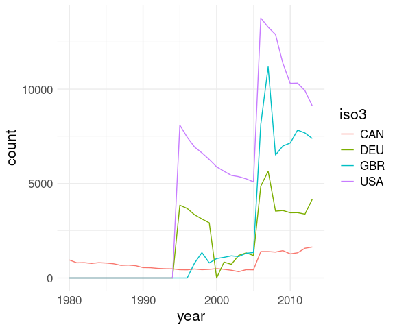
Filling In Omitted Values
The Refugee Processing Center provides information from the United States Refugee Admissions Program (USRAP), including arrivals by state and nationality.
Three files are available locally:
data from early January 2017;
data from early April 2017.
data from early March 2018.
These are Excel spread sheets.
Reading in the third file, with data for October 2017 through February 2018:
ref_url <-
    "http://homepage.stat.uiowa.edu/~luke/data/Arrivals-2018-03-05.xls"
ref_file <- "Arrivals-2018-03-05.xls"
if (! file.exists(ref_file))
    download.file(ref_url, ref_file)

library(readxl)
ref <- read_excel(ref_file, skip = 16) ## skip header
ref <- head(ref, -2) ## drop last two rows
names(ref)[1] <- "Destination"
The Destination column needs filling in (this is common in spread sheet data):
ref
## # A tibble: 500 × 18
##    Destination Nationality   Oct   Nov   Dec   Jan   Feb   Mar   Apr   May   Jun
##    <chr>       <chr>       <dbl> <dbl> <dbl> <dbl> <dbl> <dbl> <dbl> <dbl> <dbl>
##  1 Alabama     <NA>            0     0     3     1     4     0     0     0     0
##  2 <NA>        Dem. Rep. …     0     0     3     0     4     0     0     0     0
##  3 <NA>        El Salvador     0     0     0     1     0     0     0     0     0
##  4 Alaska      <NA>            9     2     6     0     0     0     0     0     0
##  5 <NA>        Russia          0     0     6     0     0     0     0     0     0
##  6 <NA>        Ukraine         9     2     0     0     0     0     0     0     0
##  7 Arizona     <NA>           26    47    71    73   110     0     0     0     0
##  8 <NA>        Afghanistan     0     1    14    10    17     0     0     0     0
##  9 <NA>        Algeria         0     0     0     0     1     0     0     0     0
## 10 <NA>        Bhutan          2     3     8     2     0     0     0     0     0
## # ℹ 490 more rows
## # ℹ 7 more variables: Jul <dbl>, Aug <dbl>, Sep <dbl>, Cases <dbl>, Inds <dbl>,
## #   State <dbl>, U.S. <dbl>
Fill down the Destination:
ref_clean <-
    fill(ref, Destination)
ref_clean
## # A tibble: 500 × 18
## Destination Nationality Oct Nov Dec Jan Feb Mar Apr May Jun
## <chr> <chr> <dbl> <dbl> <dbl> <dbl> <dbl> <dbl> <dbl> <dbl> <dbl>
## 1 Alabama <NA> 0 0 3 1 4 0 0 0 0
## 2 Alabama Dem. Rep. … 0 0 3 0 4 0 0 0 0
## 3 Alabama El Salvador 0 0 0 1 0 0 0 0 0
## 4 Alaska <NA> 9 2 6 0 0 0 0 0 0
## 5 Alaska Russia 0 0 6 0 0 0 0 0 0
## 6 Alaska Ukraine 9 2 0 0 0 0 0 0 0
## 7 Arizona <NA> 26 47 71 73 110 0 0 0 0
## 8 Arizona Afghanistan 0 1 14 10 17 0 0 0 0
## 9 Arizona Algeria 0 0 0 0 1 0 0 0 0
## 10 Arizona Bhutan 2 3 8 2 0 0 0 0 0
## # ℹ 490 more rows
## # ℹ 7 more variables: Jul <dbl>, Aug <dbl>, Sep <dbl>, Cases <dbl>, Inds <dbl>,
## # State <dbl>, U.S. <dbl>Drop the totals:
ref_clean <-
    fill(ref, Destination) |>
    filter(! is.na(Nationality))
ref_clean
## # A tibble: 451 × 18
## Destination Nationality Oct Nov Dec Jan Feb Mar Apr May Jun
## <chr> <chr> <dbl> <dbl> <dbl> <dbl> <dbl> <dbl> <dbl> <dbl> <dbl>
## 1 Alabama Dem. Rep. … 0 0 3 0 4 0 0 0 0
## 2 Alabama El Salvador 0 0 0 1 0 0 0 0 0
## 3 Alaska Russia 0 0 6 0 0 0 0 0 0
## 4 Alaska Ukraine 9 2 0 0 0 0 0 0 0
## 5 Arizona Afghanistan 0 1 14 10 17 0 0 0 0
## 6 Arizona Algeria 0 0 0 0 1 0 0 0 0
## 7 Arizona Bhutan 2 3 8 2 0 0 0 0 0
## 8 Arizona Burma 6 3 7 1 9 0 0 0 0
## 9 Arizona Burundi 0 0 0 5 7 0 0 0 0
## 10 Arizona Colombia 0 0 2 0 0 0 0 0 0
## # ℹ 441 more rows
## # ℹ 7 more variables: Jul <dbl>, Aug <dbl>, Sep <dbl>, Cases <dbl>, Inds <dbl>,
## # State <dbl>, U.S. <dbl>Pivot to a tidier form with one row per month:
ref_clean <-
    fill(ref, Destination) |>
    filter(! is.na(Nationality)) |>
    pivot_longer(
        Oct : Sep,
        names_to = "month",
        values_to = "count")
ref_clean
## # A tibble: 5,412 × 8
## Destination Nationality Cases Inds State U.S. month count
## <chr> <chr> <dbl> <dbl> <dbl> <dbl> <chr> <dbl>
## 1 Alabama Dem. Rep. Congo 2 7 0.875 0.000811 Oct 0
## 2 Alabama Dem. Rep. Congo 2 7 0.875 0.000811 Nov 0
## 3 Alabama Dem. Rep. Congo 2 7 0.875 0.000811 Dec 3
## 4 Alabama Dem. Rep. Congo 2 7 0.875 0.000811 Jan 0
## 5 Alabama Dem. Rep. Congo 2 7 0.875 0.000811 Feb 4
## 6 Alabama Dem. Rep. Congo 2 7 0.875 0.000811 Mar 0
## 7 Alabama Dem. Rep. Congo 2 7 0.875 0.000811 Apr 0
## 8 Alabama Dem. Rep. Congo 2 7 0.875 0.000811 May 0
## 9 Alabama Dem. Rep. Congo 2 7 0.875 0.000811 Jun 0
## 10 Alabama Dem. Rep. Congo 2 7 0.875 0.000811 Jul 0
## # ℹ 5,402 more rowsTop 5 destination states:
group_by(ref_clean, Destination) |>
    summarize(count = sum(count)) |>
    ungroup() |>
    slice_max(count, n = 5)
## # A tibble: 5 × 2
##   Destination count
##   <chr>       <dbl>
## 1 Ohio          750
## 2 Texas         602
## 3 Washington    562
## 4 California    545
## 5 New York      540
Top 5 origin nationalities:
group_by(ref_clean, Nationality) |>
    summarize(count = sum(count)) |>
    ungroup() |>
    slice_max(count, n = 5)
## # A tibble: 5 × 2
##   Nationality     count
##   <chr>           <dbl>
## 1 Dem. Rep. Congo  1968
## 2 Bhutan           1884
## 3 Burma            1240
## 4 Ukraine          1021
## 5 Eritrea           648
Completing Missing Factor Level Combinations
This example is based on a blog post using data from the Significant Earthquake Database.
The data used is a selection for North America and Hawaii.
Reading in the data:
if (! file.exists("earthquakes.tsv"))
    download.file("http://homepage.stat.uiowa.edu/~luke/data/earthquakes.tsv",
                  "earthquakes.tsv")
eq <- read.table("earthquakes.tsv",
                 header = TRUE,
                 sep = "\t")
eq <- as_tibble(eq)
select(eq, STATE, everything())
## # A tibble: 254 × 47
## STATE I_D FLAG_TSUNAMI YEAR MONTH DAY HOUR MINUTE SECOND FOCAL_DEPTH
## <chr> <int> <chr> <int> <int> <int> <int> <int> <dbl> <int>
## 1 HI 6697 Tsu 1500 NA NA NA NA NA NA
## 2 MA 6013 Tsu 1668 4 13 NA NA NA NA
## 3 OR 9954 Tsu 1700 1 27 5 0 NA NA
## 4 MA 5828 Tsu 1755 11 18 9 11 35 NA
## 5 AK 5926 Tsu 1788 7 21 NA NA NA NA
## 6 AK 5927 Tsu 1788 8 6 NA NA NA NA
## 7 AK 7057 Tsu 1792 NA NA NA NA NA NA
## 8 CA 5857 Tsu 1806 3 25 8 NA NA NA
## 9 AR 1594 Tsu 1811 12 16 8 15 NA NA
## 10 AR 7058 Tsu 1811 12 16 14 15 NA NA
## # ℹ 244 more rows
## # ℹ 37 more variables: EQ_PRIMARY <dbl>, EQ_MAG_MW <dbl>, EQ_MAG_MS <dbl>,
## # EQ_MAG_MB <dbl>, EQ_MAG_ML <dbl>, EQ_MAG_MFA <dbl>, EQ_MAG_UNK <dbl>,
## # INTENSITY <int>, COUNTRY <chr>, LOCATION_NAME <chr>, LATITUDE <dbl>,
## # LONGITUDE <dbl>, REGION_CODE <int>, DEATHS <int>, DEATHS_DESCRIPTION <int>,
## # MISSING <lgl>, MISSING_DESCRIPTION <lgl>, INJURIES <int>,
## # INJURIES_DESCRIPTION <int>, DAMAGE_MILLIONS_DOLLARS <dbl>, …Some STATE entries are blank, but the location name identifies the state:
filter(eq, STATE == "") |>
    select(STATE, LOCATION_NAME)
## # A tibble: 9 × 2
##   STATE LOCATION_NAME
##   <chr> <chr>
## 1 ""    MONTANA:  CLARKSTON VALLEY
## 2 ""    ILLINOIS:  WEST SALEM
## 3 ""    NEVADA:  FALLON
## 4 ""    CALIFORNIA:  OCOTILLO
## 5 ""    COLORADO:  PAONIA
## 6 ""    ALASKA: ALEUTIAN ISLANDS: FOX ISLANDS
## 7 ""    OKLAHOMA:  SPARKS
## 8 ""    OKLAHOMA:  SPARKS, PRAGUE
## 9 ""    TEXAS:  WEST
One way to fix this:
badidx <- which(eq$STATE == "")
badstate <- sub(":.*", "",
                eq$LOCATION_NAME[badidx])
eq$STATE[badidx] <-
    state.abb[match(tolower(badstate),
                    tolower(state.name))]
Add full state names as a factor:
states <- data.frame(STATE = state.abb,
                     STATE_NAME = state.name)
eq <- left_join(eq, states, "STATE")
eq <- mutate(eq,
             STATE_NAME = factor(STATE_NAME,
                                 state.name))
Look at total number of earthquakes by state:
tbl <- count(eq, STATE_NAME)
head(tbl, 6)
## # A tibble: 6 × 2
##   STATE_NAME      n
##   <fct>       <int>
## 1 Alabama         1
## 2 Alaska         78
## 3 Arkansas        2
## 4 California    100
## 5 Colorado        2
## 6 Connecticut     1
library(forcats)
pb <- ggplot(tbl, aes(y = fct_rev(STATE_NAME), x = n)) +
geom_col() +
thm +
theme(axis.title.y = element_blank())
ps <- ggplot(tbl, aes(y = fct_rev(STATE_NAME), x = n)) +
geom_point() +
geom_segment(aes(xend = 0, yend = fct_rev(STATE_NAME))) +
thm +
theme(axis.title.y = element_blank())
pb | ps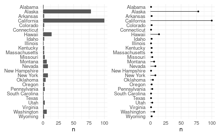
Many states, including Iowa, are missing.
Their counts should be zero.
This often impacts visualizations.
complete() can be used to fill in the zero values.
tbl <-
    count(eq, STATE_NAME) |>
    complete(STATE_NAME, fill = list(n = 0))
tbl
## # A tibble: 50 × 2
##    STATE_NAME      n
##    <fct>       <int>
##  1 Alabama         1
##  2 Alaska         78
##  3 Arizona         0
##  4 Arkansas        2
##  5 California    100
##  6 Colorado        2
##  7 Connecticut     1
##  8 Delaware        0
##  9 Florida         0
## 10 Georgia         0
## # ℹ 40 more rows
thm_ytxt_sm <- theme(axis.text.y = element_text(size = 10))
(pb %+% tbl + thm_ytxt_sm) | (ps %+% tbl + thm_ytxt_sm)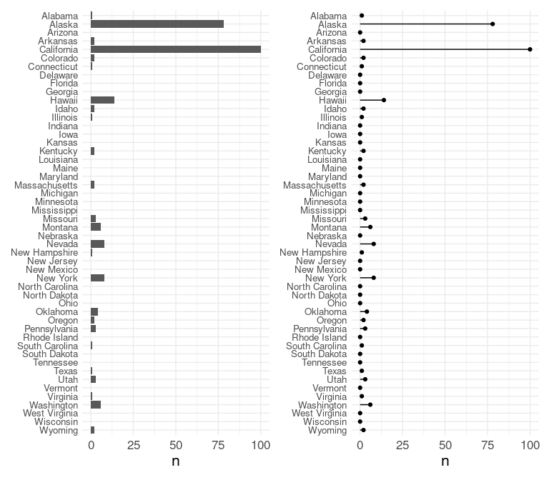
Interactive Tutorial
An interactive learnr tutorial for these notes is available.
You can run the tutorial with
STAT4580::runTutorial("dplyr")You can install the current version of the STAT4580 package with
remotes::install_gitlab("luke-tierney/STAT4580")You may need to install the remotes package from CRAN first.
Exercises
To bring in
dplyrand thempgdata, start by evaluatinglibrary(dplyr) library(ggplot2)The
selectfunction allows variables to be specified in a variety of ways. Which of the following does not produce a data frame with only the variablesmanufacturer,model,cty,hwy?select(mpg, 1:2, 7:8)select(mpg, starts_with("m"), ends_with("y"))select(mpg, 1:2, cty : hwy)select(mpg, -(displ : drv), -(fl : class))
Consider the code
library(dplyr) library(ggplot2) filter(mpg, ---) |> nrow()Which of the replacements for
---computes the number of Ford vehicles with more than 6 cylinders in thempgtable?model == "ford", cyl <= 6manufacturer == "ford" | cyl > 6manufacturer == "ford", cyl > 6manufacturer == "ford", cylinders > 6
In the 2013 NYC flights data provided by the
nycflights13package how many flights were there to Des Moines (FAA code DSM) from NYC in the first three months of 2013?- 13
- 98
- 64
- 77
To bring in
dplyrand thempgdata, start by evaluatinglibrary(dplyr) library(ggplot2)Which of the following sorts the rows for
mpgby increasingcylvalue and, within eachcylvalue sorts the rows from largest to smallesthwyvalue.arrange(mpg, desc(hwy), cyl)arrange(mpg, cyl, desc(hwy))arrange(mpg, desc(cyl), hwy)arrange(mpg, cyl, hwy)
To bring in
dplyrand theflightsdata, start by evaluatinglibrary(dplyr) library(nycflights13)The
dep_timevariable in theflightsdata set from thenycflights13package is convenient to look at (529 means 5:29 AM and 2212 means 10:12 PM), but hard to compute with. Which of the following adds variablesdep_houranddep_mincontaining hour and minute of the departure time?mutate(flights, dep_hour = dep_time %/% 60, dep_min = dep_time %% 60)mutate(flights, dep_hour = dep_time %/% 100, dep_min = dep_time %% 100)mutate(flights, dep_hour = dep_time / 100, dep_min = dep_time - dep_hour)mutate(flights, dep_hour = dep_time %/% 60, dep_min = dep_hour %% 60)
Using the
gapminderdata set, the following code computes population totals for each continent and each year:library(dplyr) library(gapminder) cpops <- group_by(gapminder, continent, year) |> summarize(pop = sum(pop)) |> ungroup()To produce a plot to compare population growth over the years for the continents it is useful to standardize the population data for each continent, for example by dividing the population values by the average population size for each continent. One way to do this is with a grouped
mutate. The first line of your result should behead(cpops_std, 1) ## # A tibble: 1 × 4 ## continent year pop stdpop ## <fct> <int> <dbl> <dbl> ## 1 Africa 1952 237640501 0.461library(ggplot2) ggplot(cpops_std, aes(x = year, y = stdpop, color = continent)) + geom_line()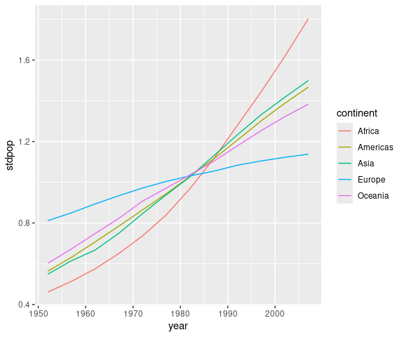
Which of the following produces the correct result:
cpops_std <- group_by(cpops, continent) |> mutate(stdpop = pop / mean(year)) |> ungroup()cpops_std <- group_by(cpops, year) |> mutate(stdpop = pop / mean(pop)) |> ungroup()cpops_std <- group_by(cpops, continent) |> mutate(stdpop = pop / mean(pop)) |> ungroup()cpops_std <- group_by(cpops, year) |> mutate(stdpop = pop / mean(year)) |> ungroup()
Another approach to the previous exercise first creates a table of population averages with
cpops_avg <- group_by(cpops, continent) |>
    summarize(avg_pop = mean(pop))
Then use a left join to add
avg_popto thecpopstable, followed by an ordinary mutate step:left_join(---) |> mutate(stdpop = pop / avg_pop)Which is the correct replacement for
---?cpops_avg, cpops, "continent"cpops, cpops_avg, "continent"cpops, cpops_avg, "year"cpops_avg, cpops, "year"