
Chapter Summary
Dynamical systems are mathematical models of "how things move." The motion of the bodies in the solar system comes to mind as a physical dynamical system. The moons and planets move in complicated ways around the sun and one another, each exerting forces on the others. Mathematical dynamical systems are broadly applicable to other kinds of "dynamics." We study discrete dynamical systems in this chapter. It appears only on the CD.
This introduction tries to answer the questions: What is a practical mathematical meaning of "dynamical system?" What does "discrete" or "continuous" mean?
In the first section, we will study two economic models of price adjustment in which the price is determined in discrete steps, p[1], p[2], p[3], .... The price at day t+1 is computed from the price at day t by an equation for the change in price.
Prices do not change during the day.
Time t moves in discrete steps, t=0,1,2,.... The change in the price is p[t+1]-p[t], and what drives this change in our first model is the "excess demand." Change in price is proportional to the amount by which demand exceeds supply:

Once we know an initial price p[0], we can rewrite the change equation in the form of a recursive definition with the unknown on one side and known values on the other,
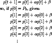

The "dynamics" in our economic models comes down to the question: Do prices tend to a limiting value, or does the economy oscillate or "blow up?" This really entails two mathematical questions. First, how does the behavior of the sequence of prices depend on the initial price? Second, how does the behavior - limiting or oscillating - depend on the parameters in the difference equation?
A practical working definition of "discrete dynamical systems" then is the study of the behavior of solutions to a difference equation as a function of the initial condition p[0] and the equation itself.
A single system (of first order) is the function that has as input the initial condition p[0] and as output the whole solution sequence


A continuous (first order, autonomous) dynamical system is the function that assigns a solution function y[t] to an initial value by means of an equation that says how the quantity changes in continuous time.
The rate of change of y is the derivative, so the analog of the difference equation is a formula for the rate of change


The whole continuous dynamical system becomes the function that assigns the solution function y[t] for
 to the initial condition through the differential equation

Since the change in a differentiable function in a small time step
 is
is

 , or
, or


20.1
The quantity consumers demand q=D[p] is a decreasing function of price, and the quantity producers are willing to supply q=S[p] is an increasing function of price.
We begin with linear supply and demand:
What happens if supply is not equal to demand? There is more than one approach to this question, so we need more economic assumptions to formulate an answer.
Suppose that we are considering a fast but not continuous adjustment.
One of the Scientific Project proposals asks you to explore a model of a baking economy.
Each morning, bakers make "Byties" and sell them at the prevailing price.
If the demand is very high, consumers buy them all up early in the day and suppliers respond the next day with more Byties - and a higher price. (Since we assume that the aggregate of producers supplies strictly in accordance with the price.) If today's Byties are selling at too high a price for consumer demand, some will go unbought, spoil, and be thrown out.
Producers will respond tomorrow by baking fewer Byties - and selling at a lower price.
If things work nicely, prices tend to a place at which producers and consumers agree.
However, it is conceivable that daily adjustments are extreme.
One day Byties are left over, so supplies and prices drop a lot, and the next day everything is sold out by 8:00 am.
Producers raise production and prices too much, and consumers respond by not buying very many.
Next, prices drop too far again... How can we capture the economic dynamics of this situation and develop mathematical criteria for "stability" of our economy? We can make the simplest possible assumption about how prices change - namely that the change in price is proportional to the amount by which demand exceeds supply,
With an initial price of p=1.20, the solution looks like Figure CD-20.3.
The dynamics in this case are that the economy adjusts production so that the price tends to equilibrium.
Suppose we want to adjust prices faster by making k=0.00135? The initial price p=0.20 produces the solution in Figure CD-20.4.
Stability of our price adjustment model apparently depends on the price adjustment constant k or the mathematical parameters
Another possible adjustment mechanism is suggested by the following different kind of economy.
Farmers decide in the spring how much corn they will plant.
Of course, each farmer does this separately, but the aggregate response is roughly an increasing supply for larger prices.
In the fall, after harvest (and all of the uncertainties of farming that our model neglects), farmers sell in a market that adjusts prices very rapidly.
For our purposes, suppose that they sell at the equilibrium price at which supply equals demand.
They are stuck with the price, but, in spring, they can adjust supply by planting more or less.
Again, for simplicity, we suppose that supply and demand are linear
The equilibrium criterion becomes
Notice that our basic difference equation is of the same mathematical form as in the first model but that the economics is different, so your experiments will lead to different conjectures economically.
In both models, the next price is an affine linear function of the current price
Apply the results of your conjectures to make predictions about the Bytie and corn economy models above; that is, re-formulate your conjectures in terms of the parameters k, aD, aS, bD, bS, in both cases.
20.2
We program the computer to compute the sequences of a discrete dynamical system by iteration of a function.
The general dynamical system
We have not used the basic formulation
The first example of the difference between using f[p] and using g[p] is in saying what an equilibrium value is dynamically.
If Pe is an equilibrium value, then when you start with p[0]=Pe or get to Pe somehow, the sequence does not change any more.
It might not always be most convenient to write a difference equation in this change form, but we can always do it by adding and subtracting p[t]. For example,
Here is a way to draw the function iteration
Now, move horizontally from the point q=p[1] on the graph of q=g[p] over to the line q=p. This point is still p[1], but next we view it as input to p[2]=g[p[1]] by moving vertically to the graph q=g[p] along p=p[1]. This gives us q=g[p[1]]=p[2].
Continue the process, alternately moving vertically from q=p to q=g[p] and horizontally back to q=p. This is simply a graphical representation of
A stable equilibrium point looks like a spider working inward toward a place at which the line q=p crosses q=g[p], and an unstable system looks like a spider working outward.
The computer program FstDscrDySy draws cobwebs as well as conventional graphs of solutions to dynamical systems.
Check your solutions to the previous exercise with it.
20.3
It is not hard to find a formula for the solution of
The stability of the system
We make a change of variables to convert our affine system into a truly linear one.
This is a very useful trick in many mathematical problems.
We are introducing a "local variable" somewhat like the one in Chapter 1. Our "local variable" is q=p-Pe, where
PROOF:
Apply the linear stability to q[t] and unchange the variables.
Show that prices in this economy stably approach
Show that prices stably approach
Problem CD-20.1
A Geometric Statement of Affine Stability
Use the CobWeb program to illustrate some examples.
20.4
The population of species with distinct generations can be modeled by discrete dynamical systems.
For example, p[t] might measure the peak population of May flies in year t. May flies hatch, live for a short period to lay eggs, and die.
The first model we consider neglects environmental limitations, such as space or food, and only concentrates on basic fertility.
The model is realistic only for the early growth of "small" populations.
Review the continuous model of algae growth in Exercise CD-28.2 and the the computer program ExpGth for comparison.
Our model is simply
Example CD-20.1
The Basic Fertility Model
where
Notice that we can express this in terms of instability of the equilibrium point Pe=0. When
If
We want to put per capita fertility at small populations together with a limited ability of the environment to support large populations.
The next model has these features.
The parameter C is a positive constant, and we are interested biologically in the case when
Example CD-20.2
The Logistic Growth Model
When p[t] is small, the term
Bugs survive in the migration model without filling the entire universe, but the biological assumptions are quite restricted.
Desert islands visited by bug-carrying birds is a narrow scope.
Our formulation of the stability theorem is the following symbolic result.
PROOF:
We use two ideas to give a symbolic proof of the geometrically obvious result of your work in Problem 20.2: The microscope or increment approximation
First, we look in the microscope, and then we show that we can look outside.
If
If we take absolute values of the estimate for the change in our dynamical system and further estimate the approximate term
Example CD-20.3
Local Stability for Logistic Systems Apply the theorem to the logistic systems
Solution:
The equilibria are Pe=0 and Pe=C. The derivative
At the equilibrium Pe=0,
At the equilibrium Pe=C,
Now, put your knowledge together on some new examples.
20.6
Section Summary
In Section CD-11.5, we studied the maximum profit of a monopoly producer, but now we want to open up the production side of our model.
The quantity of a product that producers are willing to make and the quantity that consumers are willing to buy both depend on the price of the product.
The intuition is that producers will make more when the price of their product is high, but that consumers will buy less at a higher price.

The Figure CD-20.1 shows supply and demand when

In this example, the supply and demand curves cross when p=0.93. This is the solution of the equation that says "supply equals demand."
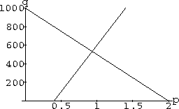
Figure CD-20.1: Linear supply and demand
20.1.1

Notice that when demand exceeds supply D[p]-S[p] is positive, and the new price is higher than the old one (assuming k is positive). If supply exceeds demand, D[p]-S[p] is negative, and the new price is lower than the old one.
In our specific linear supply and demand model, this gives us the dynamic model

or simply

with
 and
and
 Using the values above for the economic parameters aD, aS, bD, bS, and k=0.0001, beginning at a price of p[0]=0.20, we obtain the solution shown in Figure CD-20.2.
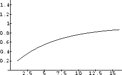
Figure CD-20.2: Prices tend to equilibrium from below
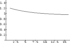
Figure CD-20.3: Prices tend to equilibrium from above
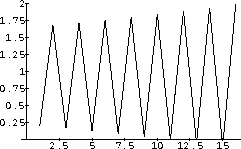
Figure CD-20.4: Bytie prices go ape
 and
and
 . We want you to explore this in an exercise below.
20.1.2

A simple equilibrium is the price p such that S[p]=D[p] 
but the dynamics of this model comes from the different times when decisions are made.
Producers set supply by last year's prices

whereas consumers decide on purchases by this year's prices

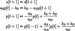
 , where
 in the first economy and
 in the second.
Some general mathematical results about the stability of affine linear dynamical systems

would apply to both of our economies (and several other applications). For example, the general equation is stable when
 as well as other cases.
This case means that the (mythical) Bytie economy is stable when
 or k=0.001 and the (simplified) corn economy is stable in the case
 or
or
 . We would really like some general rules to tell us when we have stability in terms of the parameters of our various models.
A mathematical simplification results if we first understand just the role of two parameters
 and
and
 .
.
 Experiment with the FstDscrDySy or CobWeb program to formulate a conjecture about the role of
 and
and
 in determining both the stability and limiting value of the general affine linear dynamical system given above.
Consider the following cases:
 ,
,
 , P0=100,500,1000
  ,
,
 , P0=100,500,1000
  ,
,
 , P0=100,500,1000
  ,
,
 , P0=100,500,1000
  ,
,
 , P0=100,500,1000
  ,
,
 , P0=100,500,1000
  ,
,
 , P0=100,500,1000
  ,
,
 , P0=100,500,1000
  ,
,
 , P0=100,500,1000

with P0=25. Check your work with the program FstDscrDySy.
Section Summary
There is a helpful graphical device to use in computing iterates of a discrete dynamical system.
The resulting figures look something like cobwebs, although they have nothing to do with real spiders.

recursively generates the sequence

but, written in terms of p[0], is

This looks pretty messy but is just what we get by plugging the previous value into the equation for change.
This has a simpler expression.
Let

Then, the recursion is

and the sequence of values is

the computer has a command to perform this repeated function iteration and we will use it for both discrete and continuous dynamical system computations.

for our dynamical systems because we want to emphasize the meaning of the equation as a prescription for change in the form

The connection is simply g[p]=p+f[p], but we want to formulate our results in terms of the function f[p] in order to make the clearest connection between discrete and continuous systems.
20.2.1

in other words, the change f[Pe]=0.
Definition: Equilibrium Point of a Discrete Dynamical System The number Pe is an equilibrium point for

if f[Pe]=0. In this case, the constant sequence
 is a solution of the difference equation.
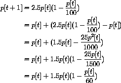
We prefer this form because of the relation to continuous systems.
In both cases, the change is zero at an equilibrium.
In this case, this means

so either Pe=0 or Pe=60.
20.2.2

Graph q=g[p] and q=p on the same axes.
Begin at the point q=P0 on the line q=p. Move vertically to the graph q=g[p] over p=P0. The value q=g(P0)=p[1] by the form of the dynamical system p[t+1]=g[p[t]].
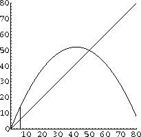
Figure CD-20.5: First iterate
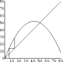
Figure CD-20.6: Two iterates

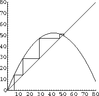
Figure CD-20.7: Five iterates
 be a solution to p[t+1]=p[t]+f[p[t]] if
 ?
?


in the change form

What is the function f[p]=? What are the equilibrium points of this system? 
How many equilibria can such a system have? What happens if
 ? How does this result compare with the conjecture you made in Exercise CD-20.1.1?


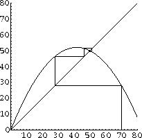
Figure CD-20.8: Six Iterates
Section Summary
The simplest (nontrivial) dynamical system we can study is
or

Plug in and do some algebra: 

is simply a question of
and this has a simple answer in five cases, which are given in Exercise CD-20.3.2. The case
 proves a basic stability result:
Theorem CD-20.1
 , the linear dynamical system
has the unique equilibrium point Pe=0. If
 , then 0 is a globally stable attractor; that is, every solution satisfies
20.3.1
Now, we want to extend our stability result to the dynamical systems of the form,

 . The value Pe is an equilibrium because
 and f[Pe]=0. We rewrite the system in terms of the local variable, q[t]=p[t]-Pe:
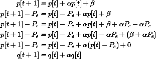
The dynamical system for q[t] is completely equivalent to the one for p[t], except that we must add or subtract Pe. The change of variables also proves
Theorem CD-20.2
 , the affine dynamical system

has the unique equilibrium point
 . If
. If
 , then Pe is a globally stable attractor; that is, every solution satisfies
 is Pe=0, draw the cobwebs, and write the closed formula solutions in the cases


(HINT: In the positive cases, you can take
 .)
.)
 and the other in the case
 .
.
 has
has
 as its unique equilibrium point if
 .
.

in terms of t,  ,
,  , and P0 is

Note that the solution to
is
 . (HINT: Resubstitute p[t]-Pe=q[t],
  . Q0=? Pe=?)
Consider the supply adjusting economy

 exactly when farmers are less excitable than consumers, aS<aD. Give an economic interpretation of the expression
 .
.
Consider the price adjustment economy driven by a multiple of excess demand: 
 under the condition that
 . Can you interpret this condition in terms of average sensitivity to price?
Rephrase the Linear Stability Theorem in terms of the cobweb diagram.
"If the dynamical system line
 crosses the line q=p at slopes between ? and ? (or angle between ? and ?), then the linear system is stable..."
Section Summary
This section extends our study of equilibria to a simple nonlinear case.

 represents the per capita fertility (or "percent" fertility as a fraction). If
 , each bug just manages to replace him or herself.
This is an average rate, so there may be many more females than males.
If
 , each bug replaces itself and also produces a new bug.
The next year there are twice as many bugs.
The second year, there are four times as many, since the doubled population doubles, and so on.
The solution to this model is

This kind of prolific growth cannot continue for very long.
The computer program ExpGth (of Chapter 28) shows that algae doubling every 3 hours would exceed the mass of all of Lake Michigan in a short period.
Whenever
 , this model eventually grows very fast.
 , we know that

 , there is an annual deficit in fertility.
For example, if
 , then the next year the population is only
 of this year's, the second only
 or 90.25% of the starting population.
As time progresses, the population goes to zero.
Mathematically,

In the mathematically stable cases where
 , the species tends to extinction.
 .
.

 is near 1, so the model behaves like our Basic Fertility Model; but, as p[t] increases, the term
 tends to zero and stops growth.
In fact, if the population ever exceeds this value p[t]>C, the term is negative
 , so p[t] "grows" negatively; in other words, p[t] declines.
Biologically speaking, we want the population to persist - that is
 - and we also seek stability - the population in harmony with the environment rather than undergoing wild oscillations in population.
 if there were migration.
Imagine bugs on a desert island where survival is difficult but where new bugs come in on birds that visit.

 in the migration model above.
If 100 new bugs migrate in each year, what is the equilibrium population?
  ?
?  and
and
 ?
?
 C=50 P0=10,60,70
  C=50 P0=10,60,70
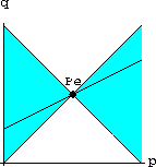

inside the sector shown, then the linear system is stable.
Theorem CD-20.3

that is, f[Pe]=0. If -2<f'[Pe]<0, then when P0 is sufficiently close to Pe, 
that is, Pe is a stable attractor for near enough initial conditions P0. 
and the local variable trick that we used in the Affine Stability Theorem.
The increment equation is used with p=Pe and
 , so it becomes

 ,
, 
Now, we localize our variable by subtracting Pe on both sides

where q=p-Pe. Any fixed number, such as m = Ave[ 1, |1+f'[Pe]|] =  , satisfies

because we have assumed that the fixed number f'[Pe] lies between -2 and 0.
 by m, then we see that for any
 ,
, 
For p[t] sufficiently close to Pe, we still have

It follows by successively plugging in and estimating that

and

so
 . (Further details of the proof are contained in the Mathematical Background.)

where
 .
.

 , so 0 is a locally stable when
 .
.
 , so C is locally stable when
 .
.


In dry conditions, the population of mythical house elder bugs in southwestern Iowa City on 15 September t years from now can be accurately estimated by taking one million times q[t], where

Show that there are three equilibria that correspond to Qe=0, Qe=1, and Qe=2. Which of these equilibria are locally stable?
20.6.1
A price adjustment model economy is explored in the Scientific Projects.
20.6.2
One of the Scientific Projects deals with a real scientific model of Sei Whales.
The question there is, "How many whales per year can we harvest without sending the population to extinction?" Unfortunately for the whales, the answer depends on their not being overexploited initially.
Mathematically, there is a positive local attracting equilibrium, but that is not the whole dynamic story.
The computer program Whales offers you some help with the simulation because the dynamical system is order 9, corresponding to the number of years it takes to produce a baby whale.
The mathematical model was derived by J.R. Beddington in a Report of the International Whaling Commission in 1978.
20.6.3
The inverse of a function y=f[x] is the function g[y] that "un-does" what f[x] does.
That is, given a value of y=y1, the value of x=x1 that makes f[x1] equal the given y1 is x1=g[y1]. For example,
 gives the angle whose tangent equals y. A method for you to use yourself to compute the inverse of complicated functions such as y=xx is given in the project on inverse functions.
The method is a discrete dynamical system such that, given a value of y1, the system converges to an equilibrium xe, with xexe=y1.