Untitled

Advanced Calculus using Mathematica

Advanced Calculus using Mathematica: NoteBook Edition is a complete text on calculus of several variables written in Mathematica NoteBooks.

Explicit 3D: Procedure 3.3.1

The Theorem on Smooth Formulas is easy to apply and it tells us that this microscopic view is true. It boils down to a procedure: compute and check that your computation makes sense. To prove smoothness when the coordinate function is given by a classical formula, verify that the formulas f[x,y], , and are valid in a rectangle about our particular point of tangency, X(x,y).

Procedure 3.3.1: Finding the Explicit Tangent Plane

Suppose f[x,y] is smooth in a neighborhood of a particular fixed X=X(x,y). To find the equation of the plane tangent to the explicit surface z=f[x,y] above X(x,y) do the following steps:

1. Compute the general symbolic total differential

(the partials are functions of x and y)

2. Calculate the specific values of the partial derivatives at the particular X(x,y), and , and write the specific total differential at this point:

d z=m·d x+n·d y

(the coefficients m and n are specific numbers)

3. (Optional) If you want the equation of the tangent line in (x,y,z)-coordinates, do the following. Say is your particular point of tangency. The local (d x,d y,d z)-coordinates are related to (x,y,z)-coordinates by , , so replace d x with , d y with , and d z wit obtaining the x-y-z-equation of the tangent to the explicit surface z=f[x,y] at

You can plot the tangent plane using the equation from Step 2 in local (d x,d y,d z)-coordinates centered on the surface at the particular (x,y,f[x,y]). The graph of this equation is an explicit plane through the (d x,d y,d z)-origin centered at the point (x,y,f[x,y]). The d x-d z-slope is m and the d y-d z-slope is n.

The result of Step 3 is an explicit (x,y,z)-plane through the fixed point with x-z-slope and y-z-slope .

Example

Find the equation of the tangent to the explicit graph above (x,y)=(1/3,2) and show that the graph is smooth near this point.

Solution

1. and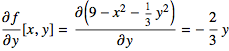

These partial derivative functions and the original f[x,y] are defined for all (x,y), so the function is smooth everywhere and has symbolic total differential

2. Substituting (x,y)=(1/3,2) in the symbolic total differential, we get the particular local equation of the tangent at (1/3,2):

3. We can replace the local variables if we want the tangent equation in x-y-z-variables,

The smoothness result of step 1 above means the plane approximates the surface “locally” or when magnified as illustrated next.

Figure 3.3.1: Zoomed in (click on graph)

In the eTopic below we explore the local linear approximation by “Zooming” with Mathematica. In Section 3.4 we will practice differentiation skills with the help of Mathematica.