University of Iowa

College of Liberal Arts and Sciences

• STAT:4580
• Syllabus
• Outline
• Homework
• Notes
• Resources
-->

Maps and Geographical Data, Continued

Simple Features

Using geom_polygon and geom_point works well for many simple applications.

For more complex applications it is best to use special spatial data structures.

An approach becoming widely adopted in many open-source frameworks for working with spatial data is called simple features.

The package sf provides a range of tools for operating with simple feature objects, such as:

• computing centroids;

• combining and intersecting objects;

• moving and expanding or shrinking objects.

Some useful vignettes in the sf package:

• Simple Features for R

• Reading, Writing and Converting Simple Features

• Manipulating Simple Feature Geometries

Other references:

• Robin Lovelace, Jakub Nowosad, Jannes Muenchow (2019; 2nd Ed. 2025). Geocomputation with R, Chapman and Hall/CRC. Also available on line.

• Mel Moreno and Mathieu Basille (2018). Drawing beautiful maps programmatically with R, sf and ggplot2, Part 1: Basics, Part 2: Layers, Part 3: Layouts.

• Claudia A Engel (2019). Using Spatial Data with R.

• Andrew Heiss (2023). Making Middle Earth maps with R.

• Taro Mieno (2023). R as GIS for Economists.

A simple utility function for obtaining map data as sf objects:

map_data_sf <- function(map, region = ".", exact = FALSE, crs = 4326, ...) {
    maps::map(map, region, exact = exact, plot = FALSE, fill = TRUE, ...) |>
        sf::st_as_sf(crs = crs) |>
        separate(ID, c("region", "subregion"), sep = ",") |>
        sf::st_transform(crs)
}

Iowa county data:

giowa_sf <- map_data_sf("county", "iowa")

This produces a special kind of data frame:

class(giowa_sf)
## [1] "sf"         "data.frame"

A key part is the geom variable:

head(giowa_sf, 4)
## Simple feature collection with 4 features and 2 fields
## Geometry type: MULTIPOLYGON
## Dimension:     XY
## Bounding box:  xmin: -94.93338 ymin: 40.60552 xmax: -91.06018 ymax: 43.51041
## Geodetic CRS:  WGS 84
##                region subregion                           geom
## iowa,adair       iowa     adair MULTIPOLYGON (((-94.24583 4...
## iowa,adams       iowa     adams MULTIPOLYGON (((-94.70992 4...
## iowa,allamakee   iowa allamakee MULTIPOLYGON (((-91.22634 4...
## iowa,appanoose   iowa appanoose MULTIPOLYGON (((-92.63009 4...

Johnson and Linn counties:

filter(giowa_sf, subregion %in% c("johnson", "linn"))
## Simple feature collection with 2 features and 2 fields
## Geometry type: MULTIPOLYGON
## Dimension:     XY
## Bounding box:  xmin: -91.82794 ymin: 41.42485 xmax: -91.34666 ymax: 42.30148
## Geodetic CRS:  WGS 84
##              region subregion                           geom
## iowa,johnson   iowa   johnson MULTIPOLYGON (((-91.34666 4...
## iowa,linn      iowa      linn MULTIPOLYGON (((-91.82221 4...

filter(giowa_sf, subregion %in% c("johnson", "linn")) |>
    ggplot(aes(fill = subregion)) +
        geom_sf() +
        coord_sf()

A basic Iowa county map using sf:

ggplot(giowa_sf) + geom_sf() + coord_sf()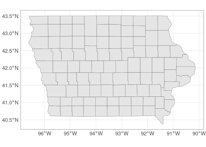

Adding wind turbine locations:

wt_IA_sf <-
    sf::st_as_sf(wt_IA,
                 coords = c("xlong", "ylat"),
                 crs = 4326)
ggplot(giowa_sf) +
    geom_sf(fill = "grey95") +
    geom_sf(aes(color = p_year),
            data = wt_IA_sf) +
    scale_color_viridis_c() +
    coord_sf()

It is possible to use geom_point but the sf coordinates may need careful adjusting:

ggplot(giowa_sf) +
    geom_sf(fill = "grey95") +
    geom_point(aes(x = xlong, y = ylat,
                   color = p_year),
               data = wt_IA) +
    scale_color_viridis_c() +
    coord_sf() +
    labs(x = NULL, y = NULL)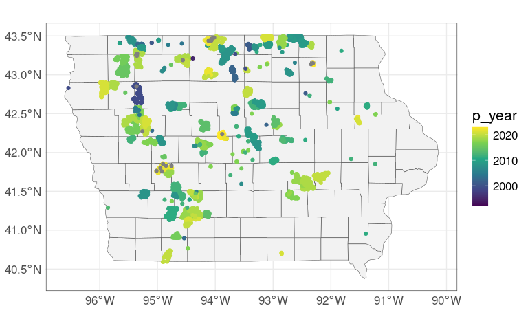

With a Stamen/Stadia map background:

library(ggmap)
register_stadiamaps(StadiaKey, write = FALSE)
m <-
    get_stadiamap(c(-97.2, 40.4, -89.9, 43.6),
                  zoom = 8,
                  maptype = "stamen_toner")
ggmap(m) +
    geom_sf(data = giowa_sf,
            fill = NA,
            inherit.aes = FALSE) +
    geom_sf(aes(color = p_year),
            data = wt_IA_sf,
            inherit.aes = FALSE) +
    scale_color_viridis_c() +
    coord_sf() +
    labs(x = NULL, y = NULL)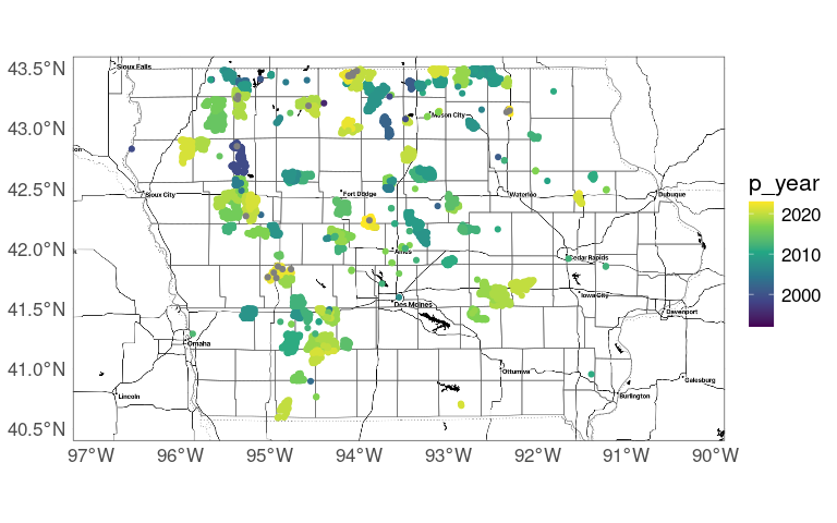

A choropleth map of population changes:

giowa_sf <- left_join(giowa_sf,
                      fipstab,
                      c("region", "subregion"))

giowa_pop_sf <-
    left_join(giowa_sf, cpop, "fips")

ggplot(giowa_pop_sf) +
    geom_sf(aes(fill = cpchange),
            show.legend = TRUE) +
    ggthemes::theme_map() +
    scale_fill_brewer(
        palette = "PRGn",
        drop = FALSE,
        guide = guide_legend(reverse = TRUE))

show.legend = TRUE is currently needed for drop = FALSE to work properly.

Proportional symbol map for 2021 Iowa county population estimates:

sf::sf_use_s2(FALSE)
iowa_pop_ctrds <-
    mutate(giowa_pop_sf,
           geom = sf::st_centroid(geom))
sf::sf_use_s2(TRUE)

ggplot(giowa_sf) +
    geom_sf() +
    geom_sf(aes(size = pop2021),
            data = iowa_pop_ctrds,
            show.legend = "point") +
    scale_size_area()

The use of sf_use_s2() can be avoided by using better map data.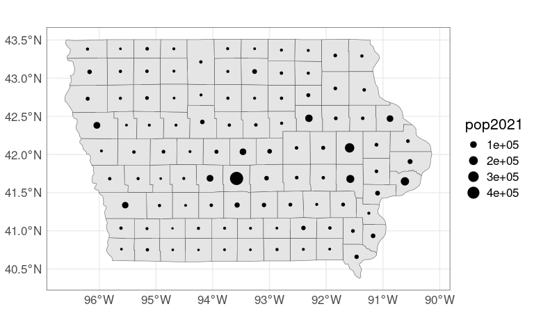

A USA county map with a Bonne projection centered on Iowa City:

gusa_sf <- map_data_sf("county")
gusa_sf <-
    left_join(gusa_sf,
              fipstab,
              c("region", "subregion"))
gusa_pop_sf <-
    left_join(gusa_sf, cpop, "fips")
ggplot(gusa_pop_sf) +
    geom_sf(aes(fill = cpchange), size = 0.1) +
    scale_fill_brewer(
        palette = "PRGn",
        na.value = "red",
        guide = guide_legend(reverse = TRUE)) +
    coord_sf(crs = "+proj=bonne +lat_1=41.6 +lon_0=-95")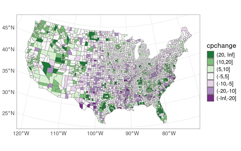

As an example of computation with sf objects we can revisit the population contour plot.

First create an sf representation of the contours (there may be better ways to do this):

ggpoly2sf <- function(poly,
                      coords = c("long", "lat"),
                      id = "group",
                      region = "region",
                      crs = 4326) {
    sf::st_as_sf(poly, coords = coords, crs = crs) |>
    group_by(!! as.name(id), !! as.name(region)) |>
    summarize(do_union = FALSE) |>
    sf::st_cast("POLYGON") |>
    ungroup() |>
    group_by(!! as.name(region)) |>
    summarize(do_union = FALSE) |>
    ungroup() |>
    sf::st_transform(crs)
}

sf_contourLines <- function(xyz, crs =  4326) {
    v <- contourLines(xyz)
    line_df <- function(i) {
        x <- v[[i]]
        x$group <- i
        as.data.frame(x)
    }
    lapply(seq_along(v), line_df) |>
        bind_rows() |>
        ggpoly2sf(coords = c("x", "y"),
                  region = "level",
                  crs = crs)
}

dsi_sf <- sf_contourLines(dsi)

This reproduces our previous plot:

ggplot(giowa_sf) +
    geom_sf() +
    geom_sf(aes(fill = level),
            data = dsi_sf,
            alpha = 0.2)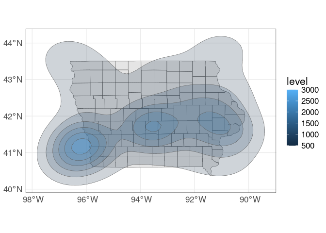

With an outline of Iowa from the maps package we can use the sf::st_intersection() function to show only the part of the contours that is within Iowa.

iowa_sf <- map_data_sf("state", "iowa")

dsi_i_sf <-
    sf::st_intersection(iowa_sf, dsi_sf)

ggplot(giowa_sf) +
    geom_sf() +
    geom_sf(aes(fill = level),
            data = dsi_i_sf,
            alpha = 0.2)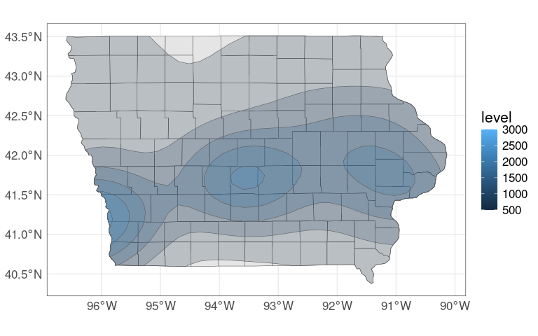

For the lower 48 states:

states_sf <- map_data_sf("state")
ds_sf <- sf_contourLines(ds)
ggplot(states_sf) +
    geom_sf() +
    geom_sf(aes(fill = level),
            data = ds_sf,
            alpha = 0.2)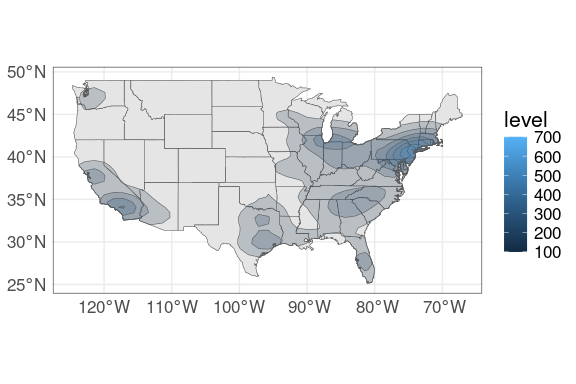

sf::sf_use_s2(FALSE)
usa_sf <- sf::st_make_valid(map_data_sf("usa"))
ds_i_sf <- sf::st_intersection(usa_sf, ds_sf)
sf::sf_use_s2(TRUE)
ggplot(states_sf) +
    geom_sf() +
    geom_sf(aes(fill = level),
            data = ds_i_sf,
            alpha = 0.2)

The cleanup steps using sf_use_s2() and st_make_valid() can be avoided by using better map data.

Shape Files

The ESRI shapefile format is a widely used vector data format for geographic information systems.

Many GIS software systems support reading shapefiles.

Shapefiles are available from many sources; for example:

• The TIGER site at the Census Bureau. The tigris package provides an R interface.

• The Natural Earth Project. The rnaturalearth package provides an R interface.

Other formats and data bases are also available. Some references:

• Paul Murrell’s R Graphics, 2nd Ed., Chapter 14.

• The CRAN Task View for Analysis of Spatial Data

• Introduction to visualising spatial data in R.

• Geocomputation with R.

World map from Natural Earth:

ne_zip <- "ne_10m_admin_0_countries.zip"
if (! file.exists(ne_zip)) {
    download.file(paste0("https://stat.uiowa.edu/~luke/data/", ne_zip),
                  ne_zip)
    unzip(ne_zip)
}
world <- sf::st_read("ne_10m_admin_0_countries.shp")
## Reading layer `ne_10m_admin_0_countries' from data source 
##   `/home/luke/writing/classes/uiowa/STAT4580/webpage/ne_10m_admin_0_countries.shp' 
##   using driver `ESRI Shapefile'
## Simple feature collection with 258 features and 168 fields
## Geometry type: MULTIPOLYGON
## Dimension:     XY
## Bounding box:  xmin: -180 ymin: -90 xmax: 180 ymax: 83.6341
## Geodetic CRS:  WGS 84
ggplot(world) +
    geom_sf(fill = "#E69F00") +
    theme(panel.background = element_rect(fill = "#56B4E950")) +
    coord_sf(crs = "+proj=moll")

State population isopleth map using shape files from the tigris package:

options(tigris_use_cache = TRUE)
ssf <- tigris::states(resolution = "20m",
                      year = 2022,
                      cb = TRUE) |>
    filter(! NAME %in% c("Alaska", "Hawaii"))

ds_sf <- sf_contourLines(ds,
                         crs = sf::st_crs(ssf))

ggplot(ssf) +
    geom_sf() +
    geom_sf(aes(fill = level),
            alpha = 0.2,
            data = sf::st_intersection(ssf,
                                       ds_sf))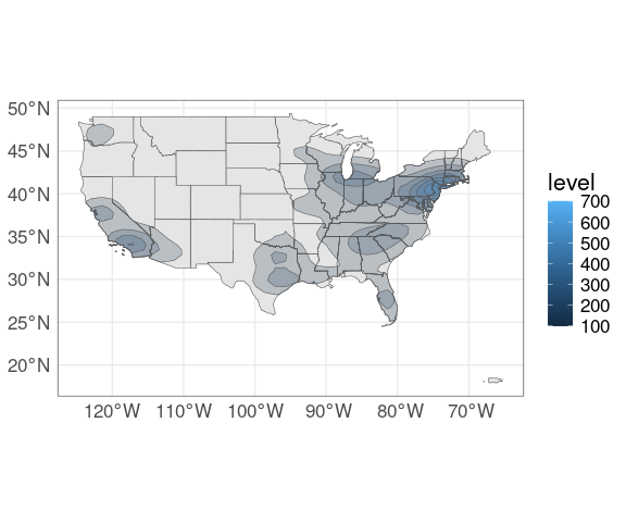

Shape Files: Census Tracts

Census Tracts are small, relatively permanent subdivisions of a county.

Census tracts generally have population sizes between 1,200 and 8,000 people.

Tracts for Iowa (state FIPS 19) for 2010:

tract_sf <- tigris::tracts(19, year = 2010)

(p <- ggplot(tract_sf) + geom_sf())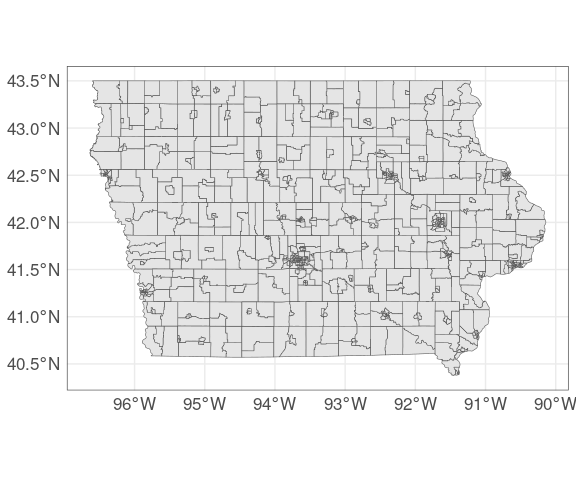

Johnson County:

p %+% filter(tract_sf, COUNTYFP == "103")

Polk County:

p %+% filter(tract_sf, COUNTYFP == "153")

Proportion of Population Without Health Insurance

A lot of data is published at the census tract level.

One example is the proportion of the population that is uninsured available from the American Community Survey.

Data from 2019 is available locally.

Download the data.

dname <- "ACS_2019_5YR_S2701"
if (! file.exists(dname)) {
    data_url <- "https://stat.uiowa.edu/~luke/data"
    aname <- paste0(dname, ".tgz")
    download.file(paste(data_url, aname, sep = "/"), aname)
    untar(aname)
    file.remove(aname)
}

Read the data.

acs_file <-
    file.path(dname,
              "ACSST5Y2019.S2701_data_with_overlays_2021-05-05T153143.csv")
acs_data_sf <- read.csv(acs_file, na.strings = "-")[-1, ] |>
    select(GEO_ID,
           name = NAME,
           population = S2701_C01_001E,
           uninsured = S2701_C05_001E) |>
    mutate(across(3:4, as.numeric)) |>
    mutate(GEO_ID = sub("1400000US", "", GEO_ID))

Merge and plot.

plot_data_sf <-
    left_join(tract_sf,
              acs_data_sf,
              c("GEOID10" = "GEO_ID"))

p <- ggplot(plot_data_sf) +
    geom_sf(aes(fill = uninsured)) +
    scale_fill_distiller(palette = "Reds",
                         direction = 1)
p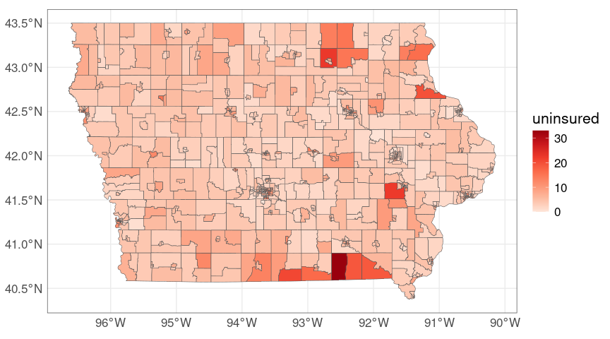

Johnson county:

p %+%
    filter(plot_data_sf, COUNTYFP == "103")

Polk county:

p %+%
    filter(plot_data_sf, COUNTYFP == "153")

For the state-wide map it may help to drop the census tract borders and add county borders:

giowa_sf <-
    tigris::counties("iowa",
                     cb = TRUE,
                     resolution = "20m")
ggplot(plot_data_sf) +
    geom_sf(aes(fill = uninsured),
            color = NA) +
    geom_sf(fill = NA,
            color = "darkgrey",
            data = giowa_sf, size = 0.2) +
    scale_fill_distiller(palette = "Reds",
                         direction = 1) +
    coord_sf()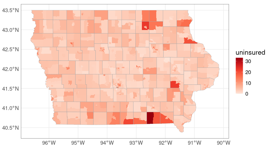

The tidycensus package provides a convenient way to work with census data, including the ACS.

library(tidycensus)
iowa_acs <- get_acs(key = CensusKey,
                    geography="tract",
                    variables = c("S2701_C01_001",
                                  "S2701_C05_001"),
                    state = "IA",
                    year = 2023,
                    geometry = TRUE,
                    output = "wide") |>
    select(GEOID,
           population = S2701_C01_001E,
           uninsured = S2701_C05_001E,
           geometry)
## Getting data from the 2019-2023 5-year ACS
## Using the ACS Subject Tables

p <- ggplot(iowa_acs) +
    geom_sf(aes(fill = uninsured)) +
    scale_fill_distiller(palette = "Reds",
                         direction = 1)

p %+% filter(iowa_acs, grepl("^19103", GEOID))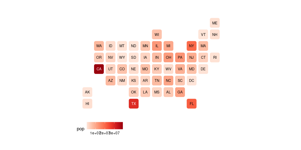

Interactive Maps: Leaflet

The leaflet package can be used to make interactive versions of these maps using the Leaflet JavaScript library for interactive maps:

library(leaflet)
lf_sf <- leaflet(sf::st_transform(plot_data_sf, 4326), width = "70%")

addPolygons(lf_sf, fillColor = ~ colorNumeric("Reds", uninsured)(uninsured),
            weight = 0.5, color = "black", fillOpacity = 0.9, opacity = 1.0,
            highlightOptions = highlightOptions(color = "white",
                                                weight = 2,
                                                bringToFront = TRUE),
            label = ~ lapply(paste0(name, "<br/>",
                                    "pct: ", uninsured, "<br/>",
                                    "pop: ", population),
                             htmltools::HTML))