Example of code profiling.
Here is an example of how a Python program might be profiled by the insertion of calls
to time(). You will need to import time in order to use the
Python time module.
def main():

 #Generating a size-million list, whose prefixes we will search
 numList = []
 for i in range(0, 1000000):
  numList.append(random.random())

 #Sorting this list
 numList.sort()


 #The input size n can range from hundred thousand to a million,
 #in increments of fifty thousand
 for n in range(100000, 1050000, 50000):
  sumBinaryTime =  0	# keeps track of the total time, over 100 trials, that binarySearch takes
  sumLinearTime = 0	# keeps track of the total time, over 100 trials, that linearSearch takes

  #We do 100 trials for each value of n
  for i in range(0, 100):
   #Generate a number to search for
   x = random.random()


   #Compute the time it takes for binarySearch
   sbt = time.time()
   binaryFound = recursiveBinarySearch(numList, 0, n-1, x)
   ebt = time.time()
   elapsedBinaryTime = ebt - sbt

   #Compute the time it takes for linearSearch
   slt = time.time()
   linearFound = linearSearch(numList, x, n)
   elt = time.time()
   elapsedLinearTime = elt - slt

   sumBinaryTime += elapsedBinaryTime
   sumLinearTime += elapsedLinearTime
  #end for-i: End of 100 trials

  print(str(sumBinaryTime) + " " + str(sumLinearTime))
I ran this program program on my Linux desktop this morning and obtained the following output. Each number is in seconds. For example, the first line is telling us that hundered binarySearch calls took about three and a half milliseconds, whereas hundred linearSearch calls took more than 3 seconds. The difference, even for arrays of size 100,000 is about three orders of magnitude.
0.0036768913269 3.34429717064
0.00372743606567 5.02832794189
0.00376796722412 6.66308569908
0.00374698638916 8.31479930878
0.00391530990601 10.0396242142
0.0039918422699 11.6610252857
0.00397181510925 13.3130259514
0.00407147407532 14.9686086178
0.00397419929504 16.6072256565
0.00412201881409 18.3236606121
0.00408315658569 19.9862177372
0.00413274765015 21.5553541183
0.00419187545776 23.4017140865
0.00413990020752 24.9976809025
0.00416684150696 26.50400424
0.00417637825012 28.1608169079
0.00421524047852 29.8988804817
0.00416707992554 31.6269822121
0.00417065620422 33.2902004719
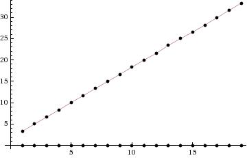
The following plot shows running times of both binary search and linear search. The x-axis is n the size of the array being search and the y-axis is the running time, in seconds. It may seem as though there is only one plot being shown, but the binary search running times are so small, relative to the linear search running times, that those running times are "hugging" the x-axis. Note how "linear" the running time plot of linear search looks. As we will soon see, this is not a surprise.
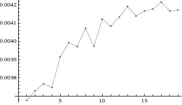
Since the above plot does not tell us much about the binar search running times,
here is a separate plot, showing just the binary search running times.
The immediately noticeable features of this plot are:
(i) the running time is not monotonically increasing and
(ii) the growth rate of the running time is falling, i.e., the running
time increases relatively fast at first and subsequently does not
increase as fast.
The profiling approach is important, but usually comes at the very end of the implementation process. But, there is a lot of analysis that happens before that and this analysis is typically of the "pen-and-paper" variety. For example, we might have to candidate algorithms A and B for a problem P. We would like to figure out which is more efficient so that we can use implement it. It takes too much time and effort to implement both and profile them. Furthermore, we have no idea of which hardware platform this will eventually be executed on. Also, we don't know how large the inputs might be for the program. Given all these uncertainities, we have no choice but to try and distinguish between A and B using a "pen-and-paper" analysis.
Features of a "pen-and-paper" analysis. The "pen-and-paper" running time analysis of algorithms and programs, does not give us absolute times. So what does it give us?