	def binarySearch(l, x):
 		first = 0
 		last = len(l)-1

 		while(first <= last):
  			mid = (first + last)/2
  			if(x == l[mid]):
   				return 1

  			if(x < l[mid]):
   				last = mid - 1
  			else:
   				first = mid + 1

 		return 0
Recall where the log2n came from. It is the number of iterations required if you start with a quantity equal to n and halve it in each iteration and stop when the quantity falls below 1. In other words, the number of iterations of the following loop:
	while(n >= 1):
		n = n/2
is roughly log2n. Similarly, if you start with a quantity whose value is 1 and double it in each iteration, stopping as soon as it exceeds n, we have a loop (see below) that executes about log2n iterations.
	prod = 1
	while(prod <= n):
		prod = prod*2
You should view these two examples as showing you "canonical" processes that execute log2n iterations. When analyzing algorithms, you should ask yourself if what the algorithm is doing is just a version of one of these processes. This phenomenon shows up a lot in computer science.
Example. The number of bits needed for a standard binary representation of n is roughly log2n. For example, 73 has the representation:
bit representation		1 0 0 1 0 0 1
bit index			6 5 4 3 2 1 0
Labeling the bits from right to left, start with index 0, we see that to represent a positive integer n, we don't need any bit with index greater than i, where 2i <= n and 2i+1 > n. By the same reasoning as in earlier examples, i turns out to be roughly log2n.
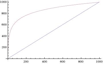
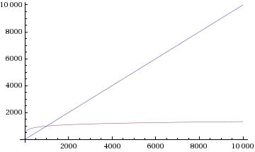
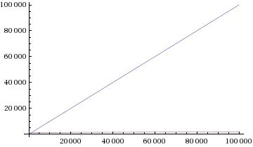
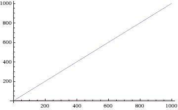
Binary search is "lightning" fast compared to linear search because its worst case running time is roughly log2n, as opposed to roughly n in the worst case for linear search.