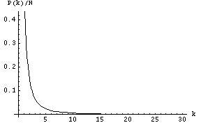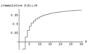


The degree distribution of graphs generated using the classical, Erdos-Renyi random graph model (see Project 1 handout) is quite different. It is a bell-shaped curve that is symmetric about the average degree. Most of the vertices have the average degree and the number of vertices having degree less than the average is about the same as the number of vertices having degree greater than the average. For a plot of the degree distribution of the Erdos-Renyi random graph see Figure 3 in this Net Wiki page on the Erdos-Renyi model.
Your first experiment will seek to determine if the random network you generated in Project 1 has a power-law degree distribution. It is now known that even though the Watts-Strogatz model appropriately models high clustering coefficient and low average path length features of social networks, it fails to generate graphs with a power-law degree distribution. Here is quote from the Net Wiki page on the Watts-Strogatz model.
Despite producing a network that is both small-world and clustered, the Watts and Strogatz Model
fails to be a good model for real networks. The WS Model is quite homogenous in degree, most
nodes have about the same degree. Real networks such as the world wide web and metabolic networks
are inhomogenous. There exist a significant number of nodes of very high degree called hubs.
So it is reasonable to expect that the random networks generated in Project 1, also, do not satisfy the power-law distribution. In fact, the starting hypothesis for your first experiment should be that the random graphs generated in Project 1 do not satisfy the power-law distribution. To perform this experiment, first add a method
int[] degreeDistribution()to the graph class. Then write a program called experiment1.java that generates random graphs as in Project 1 and outputs their degree distribution. You can fix n = 10,000 and vary the average degree between 15 and 19. For each value of average degree, generate a graph, compute its degree distribution, and plot the distribution. From the 5 resulting plots determine whether the degree distribution has the power law form. It is possible that the degree distribution plots don't have either the power law form or the Poisson form.
Now we will "rewire" some of the edges in the unit disk graph constructed in Step (1).  Suppose the vertices are
labeled 1 through n. Consider vertices in the order 1 through n and suppose that we are currently considering a
vertex v. Consider each edge {v, w} connecting v to a higher labeled vertex w. With probability p, replace edge
{v, w} by an edge {v, z} where z is picked picked uniformly at random from the set of all vertices that are not
neighbors of v (including  w).
The change we make to the rewiring step is that instead of picking z uniformly at random, it is picked in a manner that is proportional to the degrees. In other words, the higher the degree of a non-neighbor of v, the more likely it is to be picked as a vertex to connect v to. This scheme is called preferential attachment, the idea being that a vertex is more likely to connect to "popular" vertices. Here is the idea in more detail. Suppose we are considering edge {v, w} and have decided to rewire this edge. Let Z be the set of all non-neighbors of v (including w). Let D be the sum of the degrees of all vertices in Z. Then the probability of picking a vertex z in Z to connect v to should be degree(z)/D. For example, suppose that Z = {a, b, c} and the degrees of a, b, and c are 5, 3, and 7 respectively. Then the probability of picking a, b, and c should be 5/15, 3/15, and 7/15 respectively.
Create a new class called prefAttachGraph that is very similar to the smallWorldGraph class from Project 1, except that it implements the preferential attachment scheme described above, in the rewiring step. Then implement a program called experiment2.java that determines if the graphs generated by the prefAttachGraph class satisfy all three properties: (i) high clustering coefficient, (ii) small average path length, and (iii) power-law distribution. To verify the first two properties mentioned above, perform the experiments you performed for Project 1. To verify the third property, repeat Experiment 1, but with the prefAttachGraph class, rather than the smallWorldGraph class.
Start by implementing the following simple, greedy algorithm for routing a message from a given source vertex s to a given destination vertex t. The coordinates of the source vertex s and the coordinates of the destination vertex t are considered part of the message. This is analogous to how the "from address" and the "to address" usually appear on an envelope carried by the postal service.
Algorithm: Each node v that gets the message forwards the message to a neighbor who is closest to the destination t.
First, note that this algorithm does not always ensure that in each step the message gets closer to the destination. For example, the message may be at a node v which is fairly close to t, but all of v's neighbors may be further away from t. So when v forwards the message to a neighbor, the message moves away from t. This means that the algorithm may not always terminate and may cycle between nodes. Thus your implementation should have a way of detecting cycles and terminating the algorithm when a vertex is visited a second time. When the algorithm ends, successfully or unsuccessfully, you should record the following information:
We would like to compare the hop-distance and the Euclidean-distance travelled by message that reaches t successfully, with the actual shortest path hop-distance between s and t and the shortest path Euclidean-distance between s and t. You can use the breadth-first search algorithm to compute the shortest path hop-distance and Dijkstra's shortest path algorithm to compute the shortest path Euclidean-distance. A typical experiment you will perform will consist of the following steps:
Here are some more instructions on running your experiment. Let us fix N, the number of vertices in our graphs, at 10,000. Let us also fix M, the number of (s, t) pairs to be 1 million. You should run your experiment for different values of p, the probability of rewiring, and different values of D, the average degree. You might try values of D = 15, 20, 25, 30, and 35. For each (p, D) pair, generate 10 graphs to run your experiments on. The size of these experiments may be too ambitious and we might scale these down a bit, depending on how long they take to run.