HW10 Comments and Solutions

a. Verify Maximum Likelihood Estimates

The likelihood for the model is

\[\begin{equation*} L(\theta_1,\theta_2) = \frac{\exp\left\{\theta_2\sum x_i\right\}}{\theta_1^n} \exp\left\{-\sum y_i \exp\{\theta_2 x_i\}/\theta_1\right\} \end{equation*}\]

The data:

data(leuk, package = "MASS")
leuk1 <- subset(leuk, ag == "present")
x <- log(leuk1$wbc / 10000)
y <- leuk1$time

R function to compute the log-likelihood:

ll <- function(theta1, theta2) {
    n <- length(x)
    theta2 * sum(x) - n * log(theta1) - sum(y * exp(theta2 * x)) / theta1
}

The contours and the MLE:

t1 <- seq(50, 65, len = 30)
t2 <- seq(0.3, 0.6, len = 30)
g <- expand.grid(t1 = t1, t2 = t2)
z <- matrix(mapply(ll, g$t1, g$t2), 30, 30)
contour(t1, t2, z, xlab = expression(theta[1]), ylab = expression(theta[2]))
points(56.85, 0.482, col = "blue")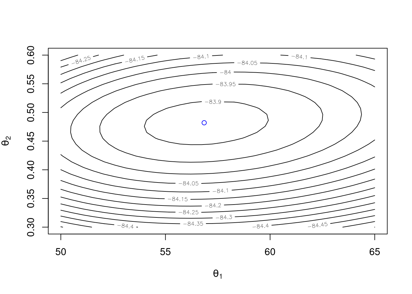

Check using optim:

optim(c(mean(y), 0), function(par) -ll(par[1], par[2]), method = "BFGS")
## $par
## [1] 56.987306  0.482118
## 
## $value
## [1] 83.87744
## 
## $counts
## function gradient 
##      130       87 
## 
## $convergence
## [1] 0
## 
## $message
## NULL

b. Marginal Posterior Density of \(\theta_2\)

Let \(\psi_1 = 1/\theta_1\). Then the posterior density of \(\psi_1,\theta_2\) is proportional to

\[\begin{equation*} f(\psi_1,\theta_2|y, x) \propto \psi_1^n\exp\left\{\theta_2\sum x_i\right\} \exp\left\{-\sum y_i \psi_1 \exp\{\theta_2 x_i\} - \psi_1/1000\right\} \end{equation*}\]

As a function of \(\psi_1\) this has the form of a Gamma density, and the unnormalized marginal posterior density of \(\theta_2\) is therefore

\[\begin{equation*} f(\theta_2|y, x) \propto \frac{\exp\left\{\theta_2\sum x_i\right\}} {\left[\sum y_i \exp\{\theta_2 x_i\} + 1/1000\right]^{n+1}} \end{equation*}\]

for \(0 < \theta_2 < 1000\).

A function to evaluate the logarithm of this unnormalized marginal density is

lf2 <- function(theta2)
    ifelse(0 < theta2 & theta2 < 1000,
           theta2 * sum(x) -
           (length(x) + 1) * log(sum(y * exp(theta2 * x)) + 1 / 1000),
           -Inf)

A plot of this density:

plot(function(x) exp(sapply(x, lf2)), 0, 1)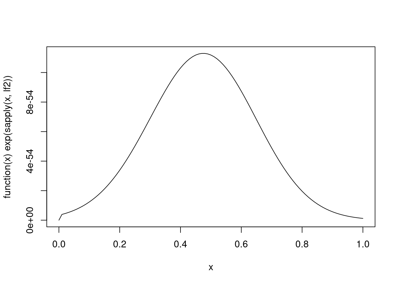

c. Sampling form the Posterior Distribution of \(\theta_2\)

Inspection of the plot shows that the mode is roughly at 0.45.

A plot of the ratio of uniforms region is obtained by

mu <- 0.45
lf2m <- lf2(mu)
tt <- seq(-4, 4, len = 1000)
u <- exp((sapply(tt + mu, lf2) - lf2m)/ 2)
v <- tt * u
plot(v, u, type = "l")
polygon(v, u, col = "grey")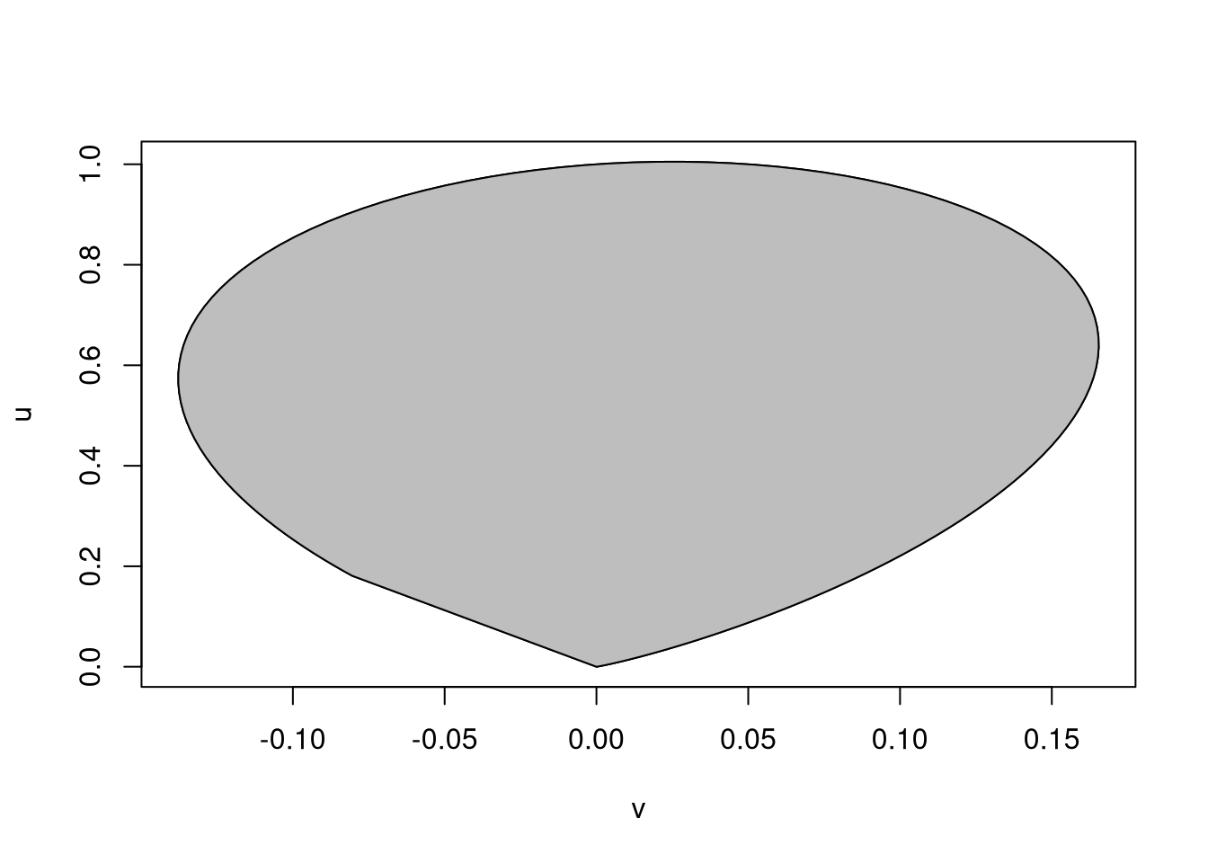

Computing the density on the log scale and subtracting the log density value at the approximate mode \(\mu\) should help with numerical stability.

Inflating the minimum and maximum of the discretized boundary values by 2% produces a rectangle that encloses the region:

vmax <- max(v) * 1.02
vmin <- min(v) * 1.02
umax <- max(u) * 1.02
plot(v, u, type = "l")
polygon(v, u, col = "grey")
rect(vmin, 0, vmax, umax)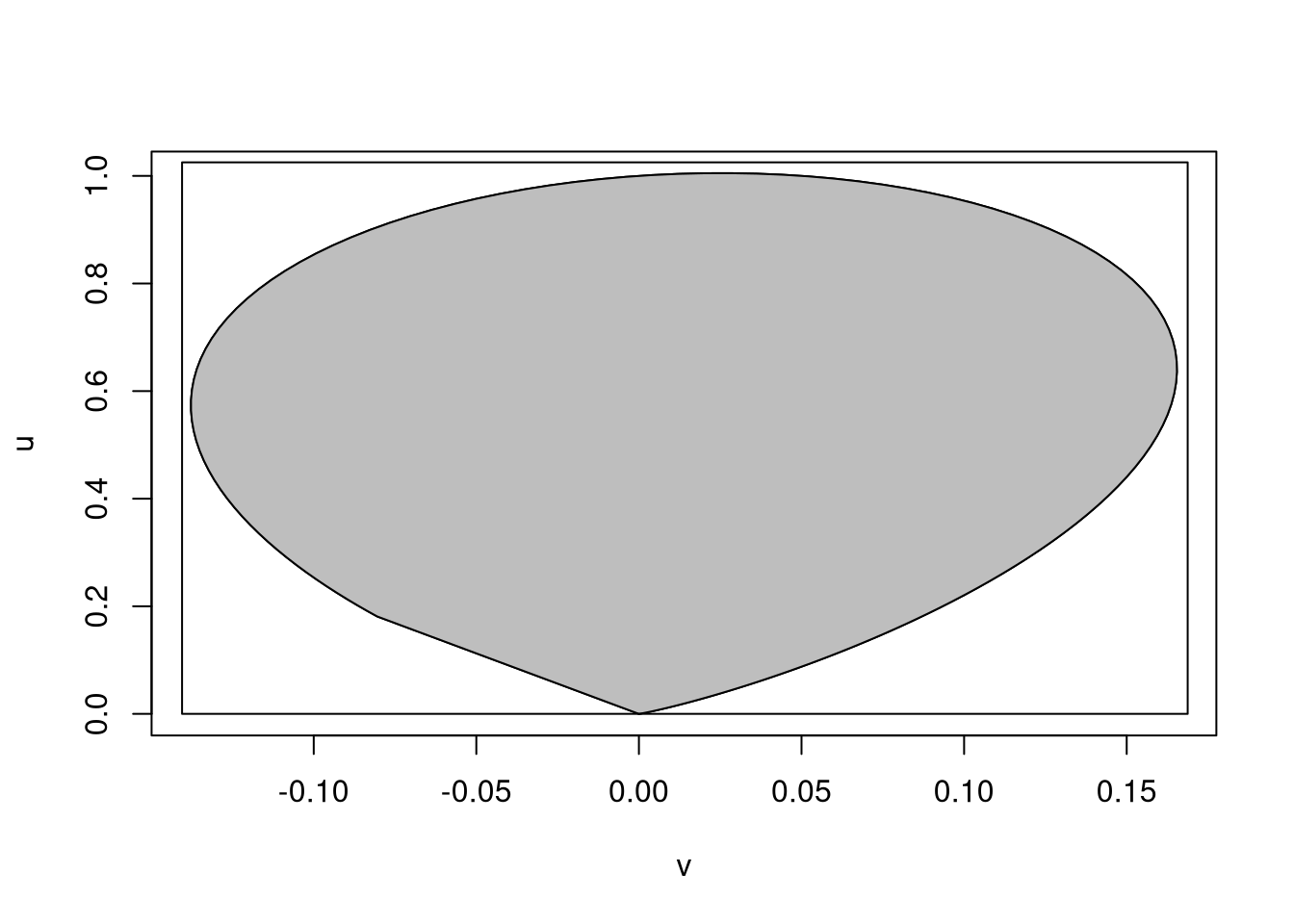

The ratio of uniforms sample is constructed by rejection sampling from this rectangle.

ru <- function(n = 10000) {
    x <- double(n)
    for (i in 1:n) {
        repeat {
            u <- runif(1, 0, umax)
            v <- runif(1, vmin, vmax)
            if (u <= exp((lf2(v / u + mu) - lf2m) / 2)) break
        }
        x[i] <- v / u
    }
    x + mu
}
theta2 <- ru(10000)

For graphical comparison of the unnormalized density and a kernel density estimate we need to scale the plots appropriately; scaling both to have maximum value of one is simplest:

d <- density(theta2)
plot(d$x, d$y / max(d$y), type = "l",
     xlab = expression(theta[1]), ylab = "")
lines(tt + mu, exp((sapply(tt + mu, lf2) - lf2m)), col = "red")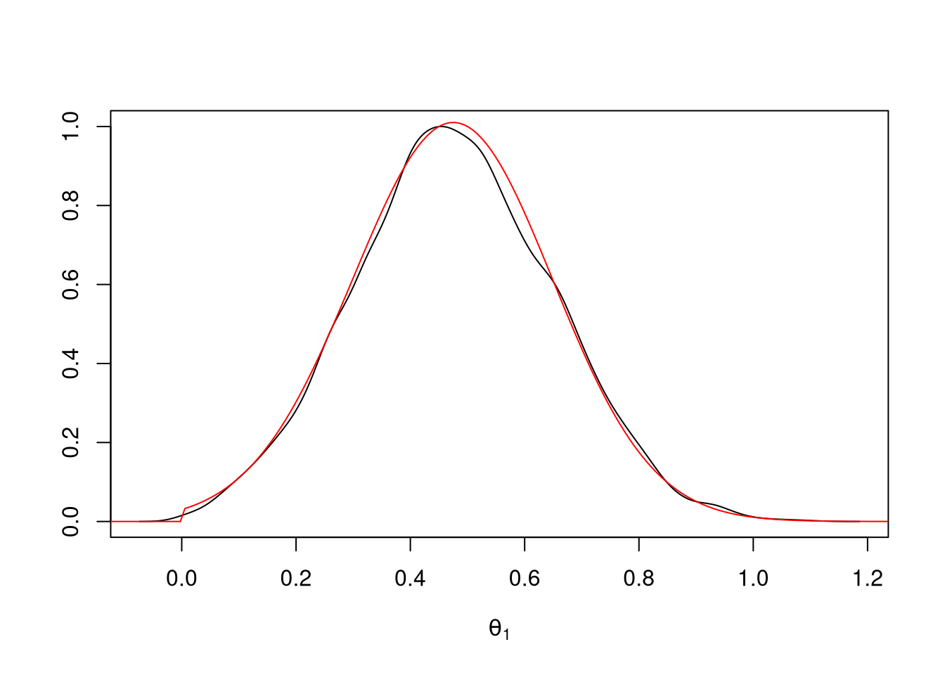

For a rejection sampling approach using a Cauchy-based envelope a little experimentation suggests:

plot(function(x) exp(sapply(x, lf2) - lf2m), 0, 1, ylim = c(0, 1.2))
xx <- seq(0, 1, len = 100)
lines(xx, dcauchy(xx, 0.475, 0.2) / 1.4, lty = 2)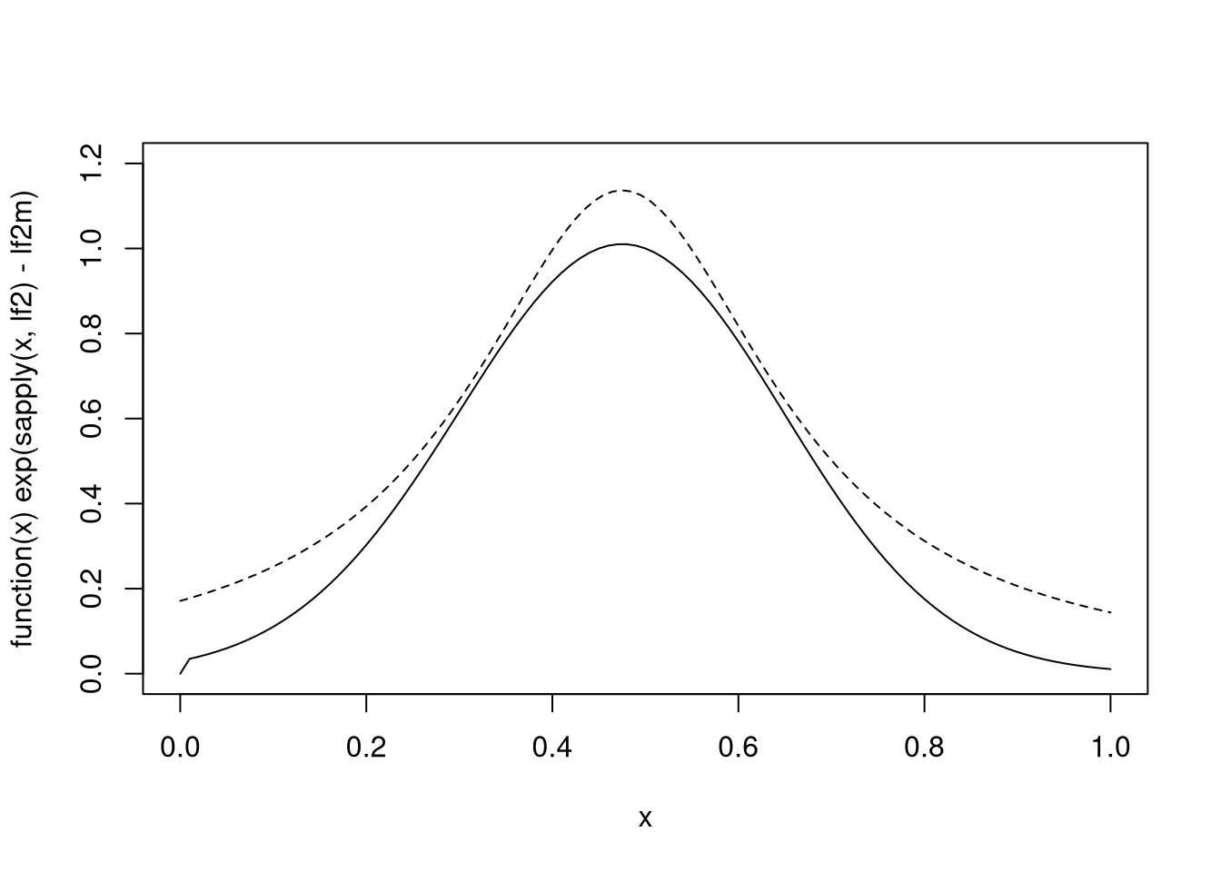

A rejection sampling function:

rej <- function(n = 10000) {
    val <- double(n)
    for (i in 1:n) {
        repeat {
            x <- rcauchy(1, 0.475, 0.2)
            y <- runif(1, 0, dcauchy(x, 0.475, 0.2))
            if (log(y) <= lf2(x) - lf2m) break
        }
        val[i] <- x
    }
    val
}
theta2_rej <- ru(10000)

Again, the density estimate matches the target density:

d <- density(theta2_rej)
plot(d$x, d$y / max(d$y), type = "l",
     xlab = expression(theta[1]), ylab = "")
lines(tt + mu, exp((sapply(tt + mu, lf2) - lf2m)), col = "red")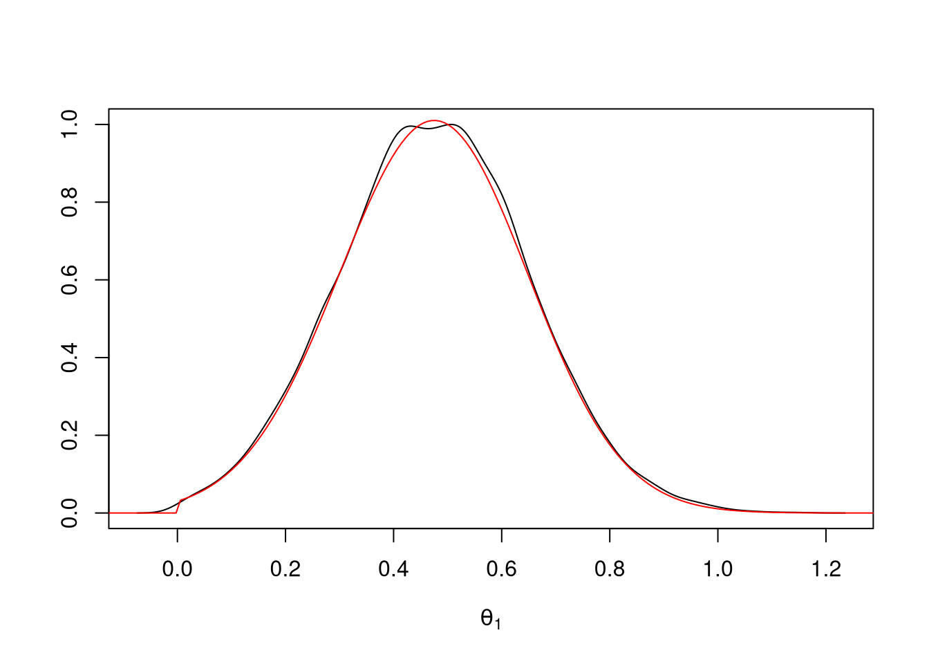

d. Sampling from the Conditional Distribution of \(\theta_1\)

The conditional distribution \(\psi_1|\theta_2\) is Gamma with exponent \(n+1\) and rate \(\sum y_i \exp\{\theta_2 x_i\} + 1/1000\).

A sample of \(\theta_1 = 1/\psi_1\) values from this conditional distribution, given the values of \(\theta_2\) obtained from the RU sampler of its marginal distribution, is generated by

theta1 <- 1/rgamma(length(theta2), length(x) + 1,
                   rate = sapply(theta2,
                                 function(t) sum(y * exp(t * x)) + 1 / 1000))

e. Estimating Posterior Moments

The estimated posterior means, variances, and covariance are computed by

mean(theta1)
## [1] 58.3533
mean(theta2)
## [1] 0.4767836
var(cbind(theta1, theta2))
##            theta1     theta2
## theta1 228.712894 0.41564799
## theta2   0.415648 0.03000078

Standard errors for the means are given by

sd(theta1) / sqrt(length(theta1))
## [1] 0.1512326
sd(theta2) / sqrt(length(theta2))
## [1] 0.001732073

and asymptotic standard errors for the variances and covariance by

sd((theta1 - mean(theta1))^2) / sqrt(length(theta1))
## [1] 4.921078
sd((theta2 - mean(theta2))^2) / sqrt(length(theta2))
## [1] 0.0004088139
sd((theta1 - mean(theta1)) * (theta2 - mean(theta2))) / sqrt(length(theta1))
## [1] 0.02898866

A plot of the estimated marginal density of \(\theta_1\) using a density estimate:

plot(density(theta1),
     main = expression(paste(bold("Marginal Density of "), theta[1])))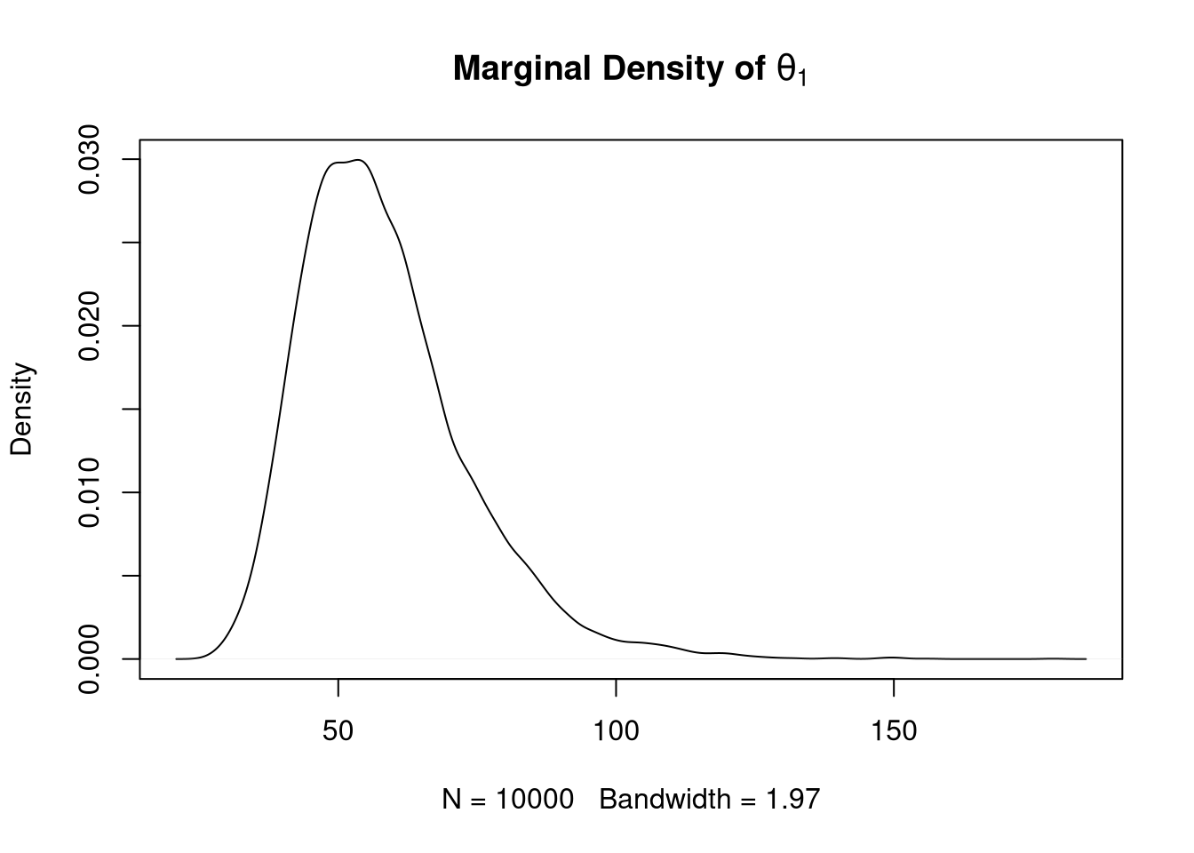

Marginal density estimates for \(\theta_1\) can be computed more accurately using Rao-Blackwellization.

The mean of \(\theta_1\) could be estimated more accurately using Rao-Blackwellization based on its inverse Gamma full conditional distribution with shape \(\alpha = n + 1\) and scale \(\beta = \sum y_i \exp\{\theta_2 x_i\} + 1/1000\). The mean of this distribution is \(\beta / (\alpha - 1)\), so a Rao-Blackwellized estimate of the posterior mean or \(\theta_1\) and its simulation standard error can be computed as

beta <- sapply(theta2, function(t) sum(y * exp(t * x)) + 1 / 1000)
mean(beta / length(x))
## [1] 58.4366
sd(beta / length(x)) / sqrt(length(beta))
## [1] 0.03409387

This full conditional distribution can also be used to obtain a more accurate estimate of the marginal posterior density of \(\theta_1\).