Next: Assignment 15
Up: 22S:193 Statistical Inference I
Previous: Assignment 14
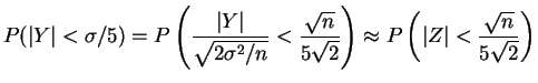
- 5.30
- Let
 . Then
So
Sinze
 ,
,
So  would do if
 . Since this
  is
quite large, it should probably be close to right.
is
quite large, it should probably be close to right.
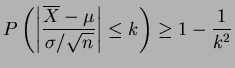
- 5.31
- Since
 ,
,
or
By Chebychev's inequality,
Taking
 means
means  or
or
 . So
. So
- First Problem
- a.
- A
 random variable
  has the same
distribution as
has the same
distribution as
 with the

 random variables. So the central limit theroem
states that
random variables. So the central limit theroem
states that
as
 .
.
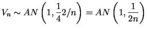
- b.
- Let
 . Now
. Now
 ,
,
 ,
,  , and
, and
 . So
. So
and thus
- c.
- Look at graphs of the densities, or at quantile plots.
- 5.62
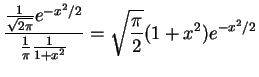
- a.
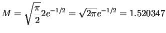
- The density ratio for a Cauchy envelope is
Since this is symmetric about the origin we can maximize for  . The ratio is maximized at the same point as its
logarithm, which is maximized at the value of
. The ratio is maximized at the same point as its
logarithm, which is maximized at the value of  that
maximizes
that
maximizes
 . The derivative of this exmpression
with respect to
. The derivative of this exmpression
with respect to  is
is
 with a root at
 . Since the derivative is decreasing on the nonnegative
half line this is a global maximum. So the maximizing value of
. Since the derivative is decreasing on the nonnegative
half line this is a global maximum. So the maximizing value of
 is
is  and
and
- b.
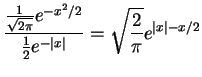
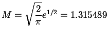
- The density ratio for a double exponential envelope is
For this is also maximized at with
- c.
- The value of
 is a little smaller for the double
exponential density than for the Cauchy density. This means the
expected number of rejections is smaller for the double
exponential. Drawing from the double exponential distribution can
be done at least as efficiently as drawing from the Caushy
distribution, so this suggests that the doulble exponential is a
slightly better choice.
is a little smaller for the double
exponential density than for the Cauchy density. This means the
expected number of rejections is smaller for the double
exponential. Drawing from the double exponential distribution can
be done at least as efficiently as drawing from the Caushy
distribution, so this suggests that the doulble exponential is a
slightly better choice.
Next: Assignment 15
Up: 22S:193 Statistical Inference I
Previous: Assignment 14
Luke Tierney
2004-12-03