Next: Assignment 12
Up: 22S:193 Statistical Inference I
Previous: Assignment 11
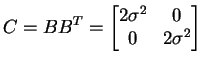
- 4.27
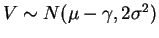
- Approach from class: Let
 be independent
standard normals and let
be independent
standard normals and let
Then
So
and
where
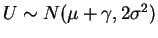 and
and
 ;
;  are independent.
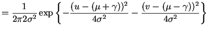
- 4.30
- a.
- The mean of
 is
is
The variance is
The covariance is
- b.
- The conditional distribution of
 , given
  is
is  . Since this conditional distribution does not depend
on
. Since this conditional distribution does not depend
on  ,
,  and
and  are independent.
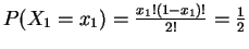
- 5.2
- a.
- Condition on
 :
:
i.e.  is geometric with
 . So for
since  is uniform on
 ![$ [0,1]$](img672.png) by the probability integral
transform. So for
by the probability integral
transform. So for

Alternative argument: For
by symmetry.
- b.
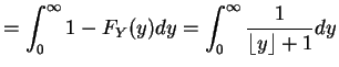
- Using
 to denote the largest integer
less than or equal to
to denote the largest integer
less than or equal to  we have
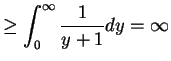
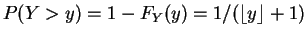 for all
  . So
. So
- 5.4
- a.
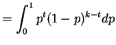
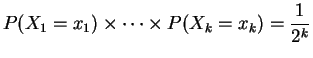
- Suppose
 are independent
Bernoulli(
are independent
Bernoulli( ). Then
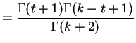
So
- b.
-
 . So
. So
For  ,
,
| |
(0,0) |
(0,1) |
(1,0) |
(1,1) |
 |
1/3 |
1/6 |
1/6 |
1/3 |
| independent |
1/4 |
1/4 |
1/4 |
1/4 |
Next: Assignment 12
Up: 22S:193 Statistical Inference I
Previous: Assignment 11
Luke Tierney
2004-12-03
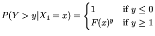
![$\displaystyle = E[F(X_{1})^{y}] = \int_{0}^{1}u^{y}du$](img669.png)