Solutions

4.15

$X,Y$ are independent,

$$X \sim (\theta) M_{X}(t) = \exp\{\theta(e^{t}-1)\}$$

$$Y \sim (\lambda) M_{Y}(t) = \exp\{\lambda(e^{t}-1)\}$$

so

$$M_{X+Y}(t) = \exp\{(\theta+\lambda)(e^{t}-1)\}$$

and thus $X+Y$ is Poisson( $\theta+\lambda$). Now

$$f_{X\vert X+Y}(x\vert z) = \frac{f_{X}(x)f_{Y}(z-x)}{f_{X+Y}(z)} = \frac{\frac{\theta^{x}}... ...x}}{(z-x)!}e^{-\lambda}} {\frac{(\theta+\lambda)^{z}}{z!}e^{-(\theta+\lambda)}}$$

$$= \frac{z!}{x!(z-x)!} \left(\frac{\theta}{\theta+\lambda}\right)^{x} \left(1-\frac{\theta}{\theta+\lambda}\right)^{z-x}$$

for $0 \le x \le z$. So $X\vert X+Y=z$ is Binomial( $z,\theta/(\theta+\lambda)$).

4.17

a.

For $y=1,2,\ldots$,

$$f_{Y}(y) = P(y-1<X<y) = e^{-(y-1)}-e^{-y}=e^{-(y-1)}(1-e^{-1})$$

So $Y$ is geometric( $p=1-e^{-1}$).

b.

$$P(X-4>x\vert Y \ge 5) = P(X-4>x\vert X \ge 4)$$

$$= \begin{cases}1 & x \le 0 e^{-x-4}/e^{-4} & x > 0 \end{cases} = \begin{cases}1 & x \le 0 e^{-x} & x > 0 \end{cases}$$

This is an exponential distrbution.

For any $t$, $X-t\vert X \ge t$ is Exponential(1).

4.36

a., b.

Suppose the $P_i$ are independent random variables with values in the unit interval and common mean $\mu$. Since the $P_i$ are independent and each $X_i$ only depends on $P_i$, the $X_i$ are marginally independent as well. Each $X_i$ takes on only the values 0 and 1, so the marginal distributions of the $X_i$ are Bernoulli with success probability

$$P(X_i = 1) = E[P(X_i=1\vert P_i)] = E[P_i] = \mu$$

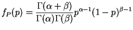
So the $X_i$ are independent Bernoulli($\mu$) random variables and therefore $Y=\sum_{i=1}^n X_i$ is Binomial($n$, $\mu$). If the $P_i$ have a Beta($\alpha$,$\beta$) distribution then $\mu = \alpha/(\alpha+\beta)$ and therefore

$$E[Y] = n \mu = n \alpha/(\alpha+\beta)$$

$$(Y) = n \mu (1 - \mu) = n \alpha \beta / (\alpha + \beta)^2$$

c.

For each $i = 1, \dots, k$

$$E[X_i] = E[E[X_i\vert P_i]] = E[n_iP_i] = n_iE[P_i] = n_i \frac{\alpha}{\alpha+\beta}$$

$$(X_i) = E[ (X_i\vert P_i)] + (E[X_i\vert P_i])$$

$$= E[n_i P_i(1-P_i)] + (n_iP_i)$$

$$= n_i E[P_i(1-P_i)] + n_i^{2} (P_i)$$

$$= n_i \int_{0}^{1}\frac{\Gamma(\alpha+\beta)}{\Gamma(\alpha)\Gamm... ...)^{\beta+1-1}dp + n_i^{2}\frac{\alpha\beta}{(\alpha+\beta)^{2}(\alpha+\beta+1)}$$

$$= n_i \frac{\Gamma(\alpha+\beta)}{\Gamma(\alpha)\Gamma(\beta)} \f... ...alpha+\beta+2)} + \frac{n_i^{2}\alpha\beta}{(\alpha+\beta)^{2}(\alpha+\beta+1)}$$

$$= \frac{n_i\alpha\beta}{(\alpha+\beta)(\alpha+\beta+1)} + \frac{n_i^{2}\alpha\beta}{(\alpha+\beta)^{2}(\alpha+\beta+1)}$$

$$= \frac{n_i\alpha\beta}{(\alpha+\beta)(\alpha+\beta+1)} \left(1+\frac{n_i}{\alpha+\beta}\right)$$

$$= n_i \frac{\alpha\beta(\alpha+\beta+n_i)}{(\alpha+\beta)^2(\alpha+\beta+2)}$$

Again the $X_i$ are marginally independent, so

$$E[Y] = \sum E[X_i] = \frac{\alpha}{\alpha+\beta}\sum_{i=1}^k n_i$$

$$(Y) = \sum (X_i) = \sum_{i=1}^k n_i \frac{\alpha\beta(\alpha+\beta+n_i)}{(\alpha+\beta)^2(\alpha+\beta+2)}$$

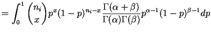
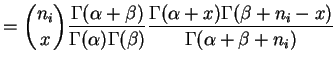
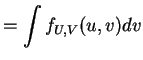
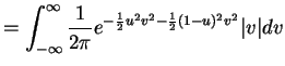
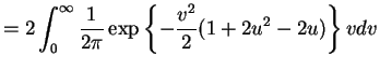
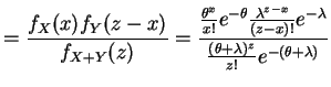
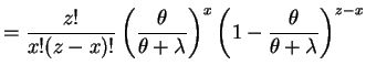
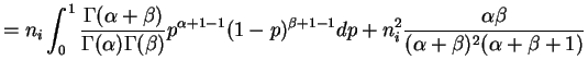
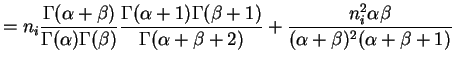
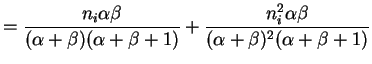
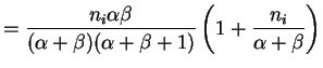
The marginal distribution of $X_i$ is called a beta-binomial distribution. The density of $P_i$ is

$$f_{P}(p) = \frac{\Gamma(\alpha+\beta)}{\Gamma(\alpha)\Gamma(\beta)} p^{\alpha-1}(1-p)^{\beta-1}$$

for $0 < p < 1$. So the PMF of $X_i$ is

$$P(X_i = x) = E[P(X_i = x\vert P_i)] = E\left[\binom{n_i}{x}P_i^x(1-P_i)^{n_i-x}\right]$$

$$= \int_{0}^{1}\binom{n_i}{x}p^{x}(1-p)^{n_i-x} \frac{\Gamma(\alpha+\beta)}{\Gamma(\alpha)\Gamma(\beta)} p^{\alpha-1}(1-p)^{\beta-1} dp$$

$$= \binom{n_i}{x}\frac{\Gamma(\alpha+\beta)}{\Gamma(\alpha)\Gamma(\beta)} \frac{\Gamma(\alpha+x)\Gamma(\beta+n_i-x)}{\Gamma(\alpha+\beta+n_i)}$$

4.21

$R^{2} \sim \chi^{2}_{2} =$   Gamma$(1,2) =$   Exponential$(2)$ and $\theta \sim$   Uniform$(0,2\pi)$.

$$X = \sqrt{R^{2}}\cos\theta$$

$$Y = \sqrt{R^{2}}\sin\theta$$

$$\mathcal{A} = (0,\infty) \times (0,2\pi)$$

$$\mathcal{B} = \mathbb{R}^{2}$$

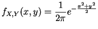
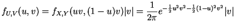
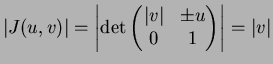
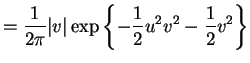
The joint density of $R^{2}, \theta$ is

$$f_{R^{2},\theta}(a,b) = \frac{1}{2}e^{-a/2}\frac{1}{2\pi}$$

for $(a,b) \in \mathcal{A}$. The inverse transformation is

$$R^{2} = X^{2}+Y^{2}$$

$$\theta = \begin{cases}\cos^{-1}\left(\frac{X}{\sqrt{X^{2}+Y^{2}}}\right)... ...0 2\pi-\cos^{-1}\left(\frac{X}{\sqrt{X^{2}+Y^{2}}}\right) & Y < 0 \end{cases}$$

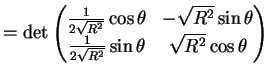
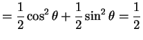
This is messy to differentiate; instead, compute

$$J^{-1} = \det \begin{pmatrix}\frac{1}{2\sqrt{R^{2}}}\cos\theta & -\sqrt{... ...ta \frac{1}{2\sqrt{R^{2}}}\sin\theta & \sqrt{R^{2}}\cos\theta \end{pmatrix}$$

$$= \frac{1}{2}\cos^{2}\theta+\frac{1}{2}\sin^{2}\theta=\frac{1}{2}$$

So $J=2$, and

$$f_{X,Y}(x,y)=\frac{1}{2\pi}e^{-\frac{x^{2}+y^{2}}{2}}$$

Thus $X,Y$ are independent standard normal variables.

4.28

a.

$$U = \frac{X}{X+Y} \mathcal{A} = \mathbb{R}^{2}$$

$$V = X+Y \mathcal{B} = \mathbb{R}^{2}$$

$$X = UV$$

$$Y = V-UV = (1-U)V$$

So

$$\vert J(u,v)\vert = \left\vert\det \begin{pmatrix}v & u -v & 1-u \end{pmatrix} \right\vert = \vert v(1-u)+uv\vert = \vert v\vert$$

Thus

$$f_{U,V}(u,v) = f_{X,Y}(uv,(1-u)v)\vert v\vert = \frac{1}{2\pi}e^{-\frac{1}{2}u^{2}v^{2}-\frac{1}{2}(1-u)^{2}v^{2}}\vert v\vert$$

and

$$f_{U}(u) = \int f_{U,V}(u,v)dv$$

$$= \int_{-\infty}^{\infty}\frac{1}{2\pi} e^{-\frac{1}{2}u^{2}v^{2}-\frac{1}{2}(1-u)^{2}v^{2}}\vert v\vert dv$$

$$= 2 \int_{0}^{\infty}\frac{1}{2\pi} \exp\left\{-\frac{v^{2}}{2}(1+2u^{2}-2u)\right\}v dv$$

$$= \frac{1}{\pi(1+2u^{2}-2u)} = \frac{1}{\pi(\frac{1}{2}+2(u-1/2)^{2})} = \frac{2}{\pi(1+4(u-1/2)^{2})}$$

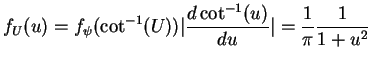
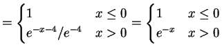
This is a Cauchy(1/2,1/2) density.

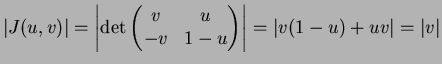
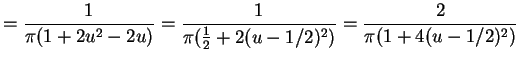
b.

$$U = X/\vert Y\vert$$

$$V = Y$$

$$X = U\vert V\vert$$

$$Y = V$$

with $\mathcal{A}=\mathcal{B}=\mathbb{R}^{2}$. So

$$\vert J(u,v)\vert = \left\vert\det \begin{pmatrix}\vert v\vert & \pm u 0 & 1 \end{pmatrix} \right\vert = \vert v\vert$$

and

$$f_{U,V}(u,v) = \frac{1}{2\pi}\vert v\vert \exp\left\{-\frac{1}{2}u^{2}v^{2}-\frac{1}{2}v^{2}\right\}$$

$$f_{U}(u) = \frac{1}{\pi(1-u^{2})}$$

4.29

a.

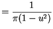
$U = X/Y = \cos \theta / \sin \theta = \cot \theta$. $\cot \theta$ is one to one on $[0,\pi)$, and periodic with period $\pi$. So $\cot \theta = \cot (\theta \mod \pi)$. Since $\psi = \theta \mod \pi$ is uniformly distributed on $[0,\pi)$ and $\cot \psi$ is one to one on $[0,\pi)$ we have $\psi = \cot^{-1}(U)$ and the density of $U$ is

$$f_U(u) = f_\psi(\cot^{-1}(U)) \vert\frac{d \cot^{-1}(u)}{du}\vert = \frac{1}{\pi}\frac{1}{1+u^2}$$

which is a standard Cauchy density.

b.

$U = 2XY/\sqrt{X^2+Y^2} = 2 R \sin\theta\cos\theta = R \sin 2\theta$. Since $\sin\theta$ and $\cos\theta$ are periodic with period $2\pi$ and since $\cos \theta = \sin (\theta +\pi/2)$ we have

$$\cos \theta = \sin(\theta+\pi/2) = \sin((\theta +\pi/2) \mod 2\pi)$$

$$\sin 2\theta = \sin (2\theta \mod 2\pi)$$

Since both $(\theta +\pi/2) \mod 2\pi$ and $2\theta \mod 2\pi$ are uniformly distributed on $[0, 2\pi)$ this shows that $\cos\theta$, $\sin\theta$ and $\sin 2\theta$ all have the same marginal distribution, and therefore $X=R\sin\theta$ has the same distribution as $R\sin 2\theta$.